Table of Contents
- Preface
- 1. Introduction
- 2. Encoding textual variation
- 3. Dissimilarity
- 4. Exploratory multivariate analysis
- 5. A survey of textual space
- 5.1. Multidimensional scaling maps
- 5.2. General remarks on the maps
- 5.3. The principal map
- 5.4. Other maps
- 5.5. Classification
- 5.6. Witness profiles
- 5.7. Cluster profiles
- 5.8. Temporal correspondence
- 5.9. Geographical correspondence
- 5.10. Results derived from the binary data matrix
- 5.11. Clustering
- 5.12. Are the clusters real?
- 5.13. Textual evolution
- 5.14. Location of the original text
- 5.15. A transmission scenario
- 5.16. Conclusion
- Bibliography
List of Figures
- 3.1. Binomial probability density for n = 44 and p = 4/44 (0.091)
- 3.2. Binomial probability density for n = 44 and p = 22/44 (0.500)
- 3.3. Binomial distribution (n = 44, p = 0.671)
- 3.4. Actual vs random agreements (B, Heb, multistate)
- 4.1. Principal components analysis (Heb, binary, UBS)
- 4.2. Classical MDS result for Australian cities
- 4.3. Classical MDS (Heb, multistate, inclusive, min. = 12, SMD)
- 4.4. Classical MDS (Heb, binary, inclusive, min. = 12, SMD)
- 4.5. Classical MDS (Heb, binary, inclusive, min. = 12, JD)
- 4.6. Classical MDS (Heb, binary, inclusive, min. = 12, ED)
- 4.7. Classical MDS (Heb, binary, exclusive, ED)
- 4.8. Biplot (Heb, binary, UBS)
- 4.9. Agglomerative clustering (single-link)
- 4.10. Agglomerative clustering (complete-link)
- 4.11. Agglomerative clustering (group-average)
- 4.12. Agglomerative clustering (Ward's criterion)
- 4.13. Divisive clustering
- 4.14. Optimal partitioning
- 5.1. Descent of clusters (binary data)
- 5.2. Descent of clusters (random data)
List of Tables
- 2.1. Types of measurement scale
- 2.2. Readings of Heb 1.3 (UBS)
- 2.3. Heb 1.3 (multistate)
- 2.4. Heb 1.3 (binary)
- 2.5. Treatment of divided witnesses
- 2.6. Example data matrices (UBS, Hebrews)
- 3.1. Frequencies of binary combinations
- 3.2. Example dissimilarity matrices (UBS, Hebrews)
- 3.3. 95% confidence interval width vs probability of disagreement (n = 44)
- 3.4. 95% confidence interval width vs probability of disagreement (n = 10)
- 3.5. 95% confidence interval width vs probability of disagreement (n = 100)
- 3.6. Maximum relative width of 95% confidence interval vs sample size (p = 1/2)
- 3.7. Mean and standard deviation for counts and proportions (binomial probability distribution)
- 3.8. Confidence intervals (normal approximation)
- 3.9. Normal approximation of 95% confidence intervals (p = 1/2)
- 3.10. Estimated minimum sample size (normal approximation, 95% confidence level)
- 3.11. Critical dissimilarity values compared (simple matching, alpha = 0.05)
- 4.1. Witnesses ordered by dissimilarity (Heb, multistate, inclusive, min. = 12, SMD)
- 4.2. Importance of principal components (Heb, binary, UBS)
- 4.3. Distances between Australian cities (km)
- 4.4. Cumulative proportions of variance (two dimensions)
- 5.1. Classical MDS maps (multistate data)
- 5.2. Witness coordinates (principal 3-D map)
- 5.3. Coordinate intervals covered by the three-dimensional principal map
- 5.4. Two band classification using the three-dimensional principal map
- 5.5. Five way partition of witnesses in the principal maps
- 5.6. Five way partition (multistate data)
- 5.7. Witness profiles
- 5.8. Five way cluster profiles (multistate data)
- 5.9. Additional witnesses ordered by dissimilarity (Heb, binary, inclusive, min. = 12, SMD)
- 5.10. Classical MDS maps (binary data)
- 5.11. Five way partition (binary data)
- 5.12. More witness profiles
- 5.13. Five way cluster profiles (binary data)
- 5.14. Ten partitions (binary data)
- 5.15. Random data matrix
- 5.16. Three-dimensional MDS maps of actual and randomly generated witnesses
- 5.17. Ten partitions (random data)
List of Examples
List of Equations
- 3.1. Simple matching distance (SMD)
- 3.2. Jaccard distance (JD)
- 3.3. Euclidean distance (ED)
- 3.4. Conversion from dissimilarity to percentage agreement
- 3.5. Conversion from percentage agreement to dissimilarity
- 3.6. Probability of reading x among all witnesses
- 3.7. Probability of random agreement (simple matching distance)
This electronic book applies certain multivariate analysis techniques to a part of the New Testament textual tradition. While the methodology is applicable to any part of the biblical text, this book uses as a case study the apparatus data from the Epistle to the Hebrews contained in the United Bible Societies' fourth edition of the Greek New Testament [UBS] (1993).
Having spent a number of years looking at the most ancient manuscripts of the Epistle to the Hebrews, my impression is that the scribal copying process that transmitted the text until the advent of mechanized printing has managed to preserve its message with a high degree of integrity. Various assertions have been made about the degree of confidence that can be placed in the biblical text, but little effort has been directed towards a quantitative assessment of its reliability. It may be that the reliability of the transmission system that delivered the texts of the apostles to us can be assessed in terms of information theory. In particular, the scribal copying process can be treated as transmission of a message through multiple channels where each channel is subject to transmission errors. According to information theory, it is possible to transmit a message through error-prone communication channels with a high degree of accuracy provided that certain conditions are met.
A first step in treating the biblical transmission process from the perspective of information theory is to break the text into a sequence of “symbols” that have been transmitted. Being language, the text naturally divides into a sequence of phrases, each composed of a sequence of one or more words. Each phrase had the potential to be corrupted at some point in the scribal transmission process. My PhD work on Hebrews discovered about two thousand places where the five thousand or so words of Hebrews differ among the thirty or so extant (i.e. surviving) manuscripts of Hebrews from the first millennium after Christ. Most of these were merely orthographic differences, reflecting the particular spelling practices of the scribes. However, a proportion involve substantive differences which affect the meaning in varying degrees from the more minor (e.g. changes of word order, presence or absence of articles) to the more major (e.g. “by the grace of God” versus “apart from God” at Heb. 2.9). In view of the fact that these thirty or so manuscripts represent a very small proportion of the total number of copies that were made in the first millennium, it may not be too far off the mark to say that any phrase that could vary (i.e. any but the simplest) did vary somewhere among the copies in a way that affected meaning, even if slightly.
Copying errors are a fact of the transmission process, as anyone who has attempted to produce a manual copy of one of the New Testament books will know. To assert that this is not so is to deny the evidence. The manuscripts themselves show that scribes and readers made alterations. These changes rarely seem to be creative exercises -- taking liberties with the text -- although a few notorious copies do display that character. In the main, the alterations are conservative attempts to clarify the meaning or to correct perceived corruptions introduced by earlier generations of copyists and readers.
This does not imply that the transmitted message is unreliable. On the contrary, looking across the full spectrum of extant copies shows that all preserve substantially the same message. If I produced translations of even the most diverse extant copies (say P46 and K), an audience would be hard-pressed to detect the differences between them. Of the differences noticed, most would be placed into the categories of “saying the same thing in a different way” or “not worth mentioning.” At the level of significance and meaning, my impression is that the scribal transmission process has preserved the message of the apostlic generation with a high degree of reliability. I believe that the message is trustworthy.
Those of us who are concerned with the minute details of the textual tradition nevertheless seek to understand the history of its transmission. This book seeks to draw the broad outlines of the textual tradition of Hebrews by means of multivariate analysis. It does so by considering variation units, calculating “distances” between witnesses on the basis of their readings within these variation units, then applying various multivariate analysis techniques to visualise the relative dispositions of the witnesses. Being statistical modes of analysis, it is not necessary to examine every variation unit in order to gain useful insights. Instead, a mere sample such as found in the apparatus of the UBS Greek New Testament can be analysed to obtain results.
Originally, I intended to include chapters on simulation of the copying process and on applying information theory to the problem of understanding the textual tradition. However, I have now decided to treat those topics separately at a future time, if it pleases God. This book is therefore restricted to exploring the application of multivariate analysis techniques alone. Being based on a sample of one part of the biblical textual tradition, all of the results have a provisional nature. Furthermore, the strategy employed to interpret results in chapter five reflects my thinking at the time it was written, which was 2009. Since that time I've been given the opportunity to explore comprehensive data for the General Letters thanks to the Institute for New Testament Textual Research (INTF) in Münster, Germany. New insights gained through this exploration have further influenced my interpretation of the results.[1]
Let the reader be warned that I am a stumbling amateur in the fields of statistics. More experienced practitioners will probably find fault with aspects of what I do in the chapters to come. The entire study represents an initial foray into unfamiliar territory. I hope that others will find its methods useful in understanding the data we contend with in the field of biblical textual research.
This research has been done at the expense of my wife, Eliane, and our children, Isabella and Joshua. They are a great blessing from God and bring me much joy. I am in debt to those who developed the R statistical language and environment. I doubt whether I would have made much progress in the statistical analysis without such a powerful and comprehensive tool. Gerald Donker influenced this book in a number of ways through discussions we had about multivariate analysis of New Testament textual data. Firstly, he suggested using the RGL plotting library to produce three-dimensional representations of multidimensional scaling maps. He also encouraged me to develop a less stringent strategy for dealing with missing data, allowing more witnesses to be included in a typical analysis. Finally, Gerald's comments swayed my thinking on estimating the margin of error associated with a witness location in a multidimensional scaling map.
Errors and infelicities are my own. A “U” instead of “0” prefix has been used for majuscules throughout.[2]
This book is dedicated to Jesus Christ, who is seated at the right hand of the Majesty on High.
[1] Results obtained through multivariate analysis of various data sets, including those made available by the INTF, are published at my Views of New Testament Textual Space site, which is a work in progress.
[2] The reason for doing so was my fear that initial zeros would cause problems in processing and plotting the sigla for majuscules. I have since discovered that these fears were unwarranted.
Table of Contents
“Heaven and earth will pass away, but my words will not pass away.”
Biblical textual criticism is concerned with a fundamental question: What is the text of the Bible? As with all texts copied before the advent of mechanized printing, hand-copying has introduced novel readings. We cannot be certain of the original readings without the original documents, and none of the extant manuscripts is thought to be an autograph. Even if a manuscript were the autograph of a particular writing, we would have no way of verifying the fact today. Given this situation, the best results that critical endeavours can hope to achieve are more or less accurate approximations to primitive forms of the text.
The textual variations of the Epistle to the Hebrews recorded in the apparatus of the United Bible Societies' fourth edition of the Greek New Testament [UBS] (1993) will be used to illustrate how to apply the analytical techniques that are introduced in this study. This Epistle has enough variations to be interesting and, other things being equal, results obtained for Hebrews should be representative of the Pauline corpus, at least for the witnesses treated here.
The analysis of biblical textual variation is facilitated by use of particular data structures and a suitable computing environment. Whereas the associated calculations can be performed on a number of platforms running a variety of programs, I recommend the following:
- Hardware
Any PC that can run a recent version of Ubuntu Linux.
- Operating system
Ubuntu Linux [Ubuntu]: Being open-source, this operating system can be freely downloaded and used. It includes OpenOffice, a general purpose office suite that incorporates a spreadsheet which is useful for creating data matrices.
- Statistical and graphical packages
The R Project for Statistical Computing [R Project]: This is an open-source statistics package, available for Linux, Macintosh, and Windows operating systems. Instructions on how to install the software are provided at the R Project website. On an Ubuntu system, R is installed with this command-line instruction:
sudo apt-get
              install r-recommended
; documentation is installed withsudo apt-get install r-base-htmlandsudo apt-get install r-doc-html. To use the RGL three-dimensional plotting library, the RGL package is required:sudo apt-get install r-cran-rgl. The “ImageMagick” graphics processing program must also be installed to produce animated rotating maps:sudo apt-get install imagemagick.
This book includes a number of programs written with the R scripting language. Such a script can be run on an Ubuntu system by following these steps:
Open a terminal window (Applications: Accessories: Terminal) then navigate to a suitable directory.
Download the script to this directory (e.g.
wget http://purl.org/tfinney/ATV/scripts/diss.r).Specify parameters such as input and output files by editing the script with a text editor (e.g.
gedit diss.r &).Launch the R environment by typing
Rat the command prompt.Run the script by typing
source("<script>")at the command prompt, where<script>is the script name (e.g.source("diss.r")).
Table of Contents
- Apparatus
A means of showing the readings possessed by witnesses of a text. Printed critical editions typically have an apparatus at the base of each page.
- Binary data
Data with only two possible states, one being presence and the other absence of some trait.
- Critical edition
A reconstruction of a text with a variant textual tradition. The text is often established using critical principles such as “prefer the reading which best explains the others”, “prefer the reading with the greatest geographical distribution”, or “prefer the reading found in what seem to be the most reliable witnesses”. A critical edition usually has an apparatus to identify readings with witnesses.
- Data matrix
A rectangular array which records the states of a number of objects for a number of variables. In the case of textual data, the objects are witnesses, the variables are variation units, and the states are readings of those variation units.
- Exemplar
The documentary source used when copying a text.
- Lectionary
A collection of biblical texts used for daily Bible readings.
- Lemma
A phrase from a critical text that can be used to define the boundaries of a variation unit.
- Manuscript (MS)
A hand-copied instance of a text.
- Multistate data
Data with two or more possible states.
- Nominal data
Categorical data for which the only meaningful comparison is based on identity. It does not make sense to compare nominal data on the basis of order or magnitude.
- Quotation
A quotation of a biblical text found in the work of some author, usually a Church Father.
- Reading
A section of text found among one or more witnesses at a particular variation unit.
- Siglum
A sign used in a critical apparatus to represent a witness.
- Variation unit
A place where texts of the same work diverge. Variation units are also called variant passages.
- Vector
A sequence of elements which are typically numbers.
- Version
A translation into another language.
- Witness
An instance of a text. In the case of a biblical witness, this term refers to a manuscript, lectionary, quotation, or version.
If every copy of the biblical text ever produced were available and we knew the exemplar of each one then it would be possible to identify every place where a copy deviated from its exemplar. (Some copies may have been produced using multiple exemplars, in which case one exemplar could be deemed the major source, and deviations identified by reference to it.) In practice we have but a small fraction of the total population of copies, and in all but a handful of cases we do not know the exemplar. Under these circumstances, it is not possible to identify every textual deviation that ever occurred. However, extant copies of a particular section of the biblical text can be collated to find places where the text is known to diverge.
Before the advent of mechanized printing, copies were produced by hand. These manuscripts served as source documents for other incarnations of the text including collections of daily Bible readings known as lectionaries and quotations by various authors. Manuscripts were also used to produce versions in other languages. An individual instance of the text, whether a manuscript, lectionary, version, or quotation, is called a witness.
Each place of known divergence between witnesses is referred to as a variation unit, and each variation unit is comprised of one or more readings. A reading might consist of a word, phrase, or nothing at all if a witness has nothing at the relevant site. (In the case of versions, the reading is a back-translation.)
Variation units are often defined by reference to the text of a critical edition. In the [UBS] Greek New Testament, for example, a phrase from the text is marked as a lemma and the apparatus shows which reading stands in place of the lemma for every witness covered by the edition. The boundaries of each lemma are fairly arbitrary, being a matter of editorial preference. Another approach breaks down places where divergence occurs into binary variation units, each recording the presence or absence of some trait.
A critical apparatus often uses sigla to refer to witnesses. A siglum is usually identified with a single witness but sometimes refers to a composite that represents a group of witnesses such as Byzantine manuscripts, lectionary manuscripts, or manuscripts of a version. At least in theory, these composite forms can be resolved into individual witnesses although a given critical edition may not provide enough information to do so.
Variations can be classified in a number of ways: a substantive variant affects the meaning of the text; an orthographic variant affects scribal particulars (e.g. spelling) but not meaning; a punctuation variant affects division into sense units. Much can be gained by analysing each class of variation; however, this study restricts itself to substantive variation alone. (Analysis of substantive and orthographic variation conducted during my doctoral research [Finney 1999] points to a shared pattern of agreement among these two kinds. If orthography depends on locality then this phenomenon is evidence for the existence of local texts.)
Whereas biblical textual criticism speaks of witnesses, variation units, and readings, multivariate analysis (MVA) employs a different vocabulary. According to [Venables and Ripley] (2002 301),
Multivariate analysis is concerned with datasets that have more than one response variable for each observational or experimental unit. The datasets can be summarized by data matrices X with n rows and p columns, the rows representing the observations or cases, and the columns the variables.
The apparatus of a critical edition corresponds to the “dataset”, witnesses correspond to “cases”, variation units correspond to “variables”, and readings correspond to unique states of each variable.
A data matrix is a rectangular array of elements which are usually numbers:
| X = | x11 | x12 | ... | x1p |
| x21 | x22 | ... | x2p | |
| ... | ... | ... | ... | |
| xn1 | xn2 | ... | xnp |
It may be viewed as a set of n row vectors with p elements, p column vectors with n elements, or a matrix with n x p elements. The information contained in an apparatus can be represented as a data matrix in which rows correspond to witnesses and columns to variation units. The data matrix cell located at the intersection of a row and column indicates the reading of the corresponding witness for the corresponding variation unit. Each row represents an observation of the text at a particular date and location; each column shows the states of witnesses for a particular variation unit.
The elements of a data matrix may be classified according to the scale against which they are measured. Four types of scale are often distinguished [Everitt] (2005 2):
| Name | Description |
|---|---|
| Nominal | A categorical scale whose points have no inherent order. E.g. nationality: Australian, Brazilian, Canadian, ... |
| Ordinal | A scale whose points do have an inherent order but intervals between consecutive points on the scale are not necessarily equal. E.g. letter grade: A, B, C, ... |
| Interval | A scale with equal intervals between consecutive points and an arbitrary zero point. E.g. Celsius or Fahrenheit temperature scales. |
| Ratio | A scale with equal intervals between consecutive points and an absolute zero point. E.g. the Kelvin temperature scale. |
This table places measurement scales according to their expressive power. The only meaningful comparison for nominal measurements is whether or not they are the same. Ordinal measurements are more expressive, being able to be placed in order. In addition to having an ordinal quality, the difference between interval measurements is meaningful. A ratio scale is the most expressive: the order, difference, and ratio of measurements made against such a scale are all meaningful.
This study treats the data of the UBS textual apparatus as purely nominal. The readings of a variation unit differ, but it is meaningless to apply the mathematical operations of division or subtraction to them. One may argue that this data is ordinal because the UBS editors give priority to the first reading of each variation unit. Also, if the readings of each variation unit were somehow to be arranged in order, perhaps using a genealogical principle, then the apparatus data could be treated as ordinal.
Nominal data is encoded
prior to analysis, often by a one-to-one mapping of states to numerical
labels. Binary data has only
two states, the first signifying presence and the second absence of some
trait. By convention, presence is represented by 1 and
absence by 0. Multistate
data has two or more states. It can be encoded by assigning
a unique numeral to each state, normally starting with 1 and
proceeding with 2, 3, etc. These numerals have
no inherent significance, serving merely as labels to distinguish
different states. Being nominal data, the only comparison that makes sense
is whether two labels are the same; it does not make sense to compare the
magnitudes or order of the numerical labels that represent the states of
such data. It is always possible to convert multistate nominal data into a
binary form by resolving each variable into a group of one or more binary
variables.
Parts of the data set may be missing, as when a witness does not cover
a part of the biblical text, is fragmentary, or has an ambiguous reading.
If the reading of a witness at a particular variation unit is not known
then the corresponding element of the data matrix is not defined. Rather
than leave the element empty, it is labelled as NA, meaning
“not available”.
Missing data is different to the state of binary data that signifies
absence. In the latter, the state is defined; in the former it is not. To
illustrate, consider a piece of text in which some witnesses have the
definite article and others do not. In a binary representation, presence
of the article is labelled as 1 and absence as
0. The state of a witness which has a lacuna at the relevant
place is not defined. The corresponding cell of the data matrix is
therefore labelled as NA.
Missing data causes problems when it comes to analysis. Ideally, the state of every witness would be defined for every variation unit under examination. This is seldom the case in practice, so a strategy for dealing with missing data is required. One approach, which I call the exclusive strategy, specifies a reference witness, eliminates all variation units (i.e. columns of the data matrix) for which it is not defined, then eliminates witnesses (i.e. rows of the data matrix) which still contain missing data. The result is a reduced data matrix which is completely free of missing data.
Another approach, which I call the inclusive strategy, sets the condition that each pair of witnesses in the desired data matrix must share a minimum number of defined variation units. Through an iterative process, witnesses that cause this condition to be violated are eliminated until the processed data matrix satisfies the condition. The result is a reduced data matrix which retains more witnesses than would be the case if the exclusive strategy were used. However, witnesses within the data matrix may still have undefined variation units. A reference witness can also be specified when using the inclusive strategy, in which case columns of the original data matrix for which the reference witness are not defined are eliminated prior to beginning the iterative reduction process. In this way, the reference witness is guaranteed to be included in the resulting data matrix.
The first step in converting the information of an apparatus into a form suitable for multivariate analysis is to construct a data matrix. By convention, rows of a data matrix are devoted to cases (i.e. witnesses) and columns to variables (i.e. variation units). Consequently, the first task is to isolate the reading of every witness for every variation unit. This immediately raises two questions:
How does one define a witness?
How does one define a variation unit?
Sigla included in a typical apparatus may refer to composites: a manuscript may have a number of scribes and correctors; Greek and Latin versions of the same Church Father may have different readings; a version may have subversions (e.g. copsa, copbo, copfay) or multiple editions (e.g. vgcl, vgww, vgst); some manuscripts of a version may differ from other manuscripts or the standard edition of that version; a reading may be supported by some lectionary manuscripts but not the lectionary text of the Greek Church; a witness may have marginal readings or may even have its own critical apparatus! Ambiguous data complicates subsequent analysis so it is prudent to resolve composite witnesses into their constituents, treating the text of each scribe, corrector, subversion, edition, or distinct lectionary as a separate witness.
Even a resolved witness may have an ambiguous or uncertain reading. If so, one can ignore the witness for that variation unit, or include the most probable reading and ignore any alternatives. This is not to understate the importance of alternative readings; it is instead a constraint imposed by the methodology. Perhaps the best policy is to exclude all readings of a witness which are subject to a substantial level of doubt. This has the unfortunate consequence of removing some interesting readings from consideration. On the other hand, a strict policy of excluding ambiguous data allows more confidence to be placed in analytical results derived from what remains.
When it comes to defining variation units, one must decide between a binary or multistate representation of the data. A multistate rendition presents every variation unit as two or more mutually exclusive readings. The boundaries between variation units and the division of a variation unit into readings are determined by editors and are somewhat arbitrary. A binary representation is less arbitrary, reducing every stretch of variant text to a series of binary variation units, each characterised by presence or absence of a word or phrase. (Some multistate variation units are already binary, having only two states representing presence or absence of some word or phrase.)
The apparatus of a critical edition is typically comprised of multistate nominal data. Consequently, the question of how to define variation units is already answered if a multistate data matrix is being produced. If, however, one wishes to construct a binary data matrix — and there are good reasons for wanting to do so — every multistate variation unit of the apparatus must be resolved into a sequence of one or more binary variation units.
For the multistate case, the first reading can be represented by the
label 1, the second 2, the third
3, and so on. Alternatively, each multistate variation unit
can be resolved into a number of binary units where presence of a trait
is encoded as 1 and absence as 0. Missing or
ambiguous data is encoded as NA in both multistate and
binary data matrices.
One way to convert multistate nominal data into binary form constructs a catena (i.e. chain or sequence) from the words comprising the readings of a variation unit then marks presence or absence of each word for each witness. The catena is a superset of all readings, composed in such a way that the words of each reading can be extracted by a sequential selection of words from the catena.
Example 2.1. Binary encoding based on a superset catena (Heb 1.3, UBS)
The first variation unit that the UBS edition of The Greek New Testament presents for Hebrews concerns the wording of Heb 1.3. Three main readings are reported, two of which have subreadings:
| Reading | Witnesses |
|---|---|
| τῆς δυνάμεως αὐτοῦ, καθαρισμόν | 01 A B ... |
| τῆς δυνάμεως, δι᾽ ἑαυτοῦ καθαρισμόν (P46 αὐτοῦ) | 0243 6 ... |
| τῆς δυνάμεως αὐτοῦ, δι᾽ ἑαυτοῦ (or αὑτοῦ or αὐτοῦ) καθαρισμόν | D Hc 104 ... |
This information can be encoded as a single column of a multistate data matrix:
| Heb.1.3 | |
|---|---|
| P46 |
2
|
| 01 |
1
|
| A |
1
|
| B |
1
|
| D |
3
|
| Hc |
3
|
| 0243 |
2
|
| 6 |
2
|
| 104 |
3
|
| ... |
...
|
Alternatively, it can be converted to a binary form using a suitably constructed catena. Columns associated with words that do not vary across witnesses may be omitted as they do not contribute any information about variation among the witnesses.
| Heb.1.3.1 | Heb.1.3.2 | Heb.1.3.3 | Heb.1.3.4 | |
|---|---|---|---|---|
| αὐτοῦ | δι | ἑαυτοῦ | αὐτοῦ | |
| P46 |
0
|
1
|
0
|
1
|
| 01 |
1
|
0
|
0
|
0
|
| A |
1
|
0
|
0
|
0
|
| B |
1
|
0
|
0
|
0
|
| D |
1
|
1
|
1
|
0
|
| Hc |
1
|
1
|
1
|
0
|
| 0243 |
0
|
1
|
1
|
0
|
| 6 |
0
|
1
|
1
|
0
|
| 104 |
1
|
1
|
1
|
0
|
| ... |
...
|
...
|
...
|
...
|
This encoding method allows a more fine-grained comparison of witnesses. In a multistate representation there is no way to gauge the similarity of readings within a variation unit: two witnesses either agree or they don't, no matter how similar their readings. In a binary representation based on a superset catena, it is possible to determine the similarity of two witnesses within a variation unit. The resultant binary variation units can be compared on a case by case basis, thereby providing access to more of the information contained in the apparatus.
The same technique of constructing a superset catena can also be used to make binary data matrices from full transcriptions of witnesses. Once the transcriptions are prepared, a superset catena can be constructed from them by hand or by means of a computer algorithm. (One could use the algorithm described in my doctoral dissertation. Alternatively, the algorithm behind the “diff” utility commonly used to compare computer files may be adapted to the purpose.) By suitably processing the transcriptions, a separate data matrix can be constructed to focus on each phenomenon of interest, whether substantive variation, orthography, punctuation, accentuation, or lineation. This allows the relationships between witnesses to be examined from each of these perspectives, separately [Finney 1999].
In order to demonstrate how to encode textual data, the apparatus of the Epistle to the Hebrews in the United Bible Societies' fourth edition of the Greek New Testament [UBS] will be converted into forms suitable for subsequent analysis. The UBS apparatus is not comprehensive but is nevertheless well-suited for the present purpose because it explicitly includes the reading of each reported witness where extant. Other critical editions of the Greek New Testament cover far more textual variants. However, their economical use of space means that not every witness that supports a reading is explicitly reported in the apparatus. These editions can still be used to construct data matrices, but are a less convenient basis for doing so.
The following guidelines contain instructions for preparing multistate and binary data matrices. The extent of a data matrix is determined by the number of included witnesses and variation units. Examples constructed for this book are restricted to the witnesses and variation units contained in the UBS apparatus of the Epistle to the Hebrews. Once the data matrices are constructed, it is a simple matter to partition them into smaller blocks of variation units if investigating a phenomenon such as block mixture. If data matrices of a number of books are available, they can be combined together to investigate an entire corpus such as the Gospels or Pauline Epistles.
These guidelines relate to construction of a multistate data matrix from information contained in the UBS apparatus. Some, such as the instructions for recording witness sigla, may be varied according to taste without affecting the utility of the result.
Variation units are identified using a code based on book, chapter, and verse or verse range (e.g. Matt.1.7-8). An additional numeral is appended if more than one variation unit is recorded for a verse (e.g. Heb.1.12.1).
Readings are encoded according to their order in the apparatus. The first reading (i.e. the one preferred by the UBS editors) is coded as
1, the second as2, etc.Parenthesized witnesses (indicating a negligible difference from the attested reading) and those marked with a “vid” superscript (indicating the most probable reading) are encoded as if normal.
NA(not available) is entered when the state of a witness cannot be established beyond reasonable doubt.Each row is devoted to a single witness and each column is devoted to a single variation unit. A row is included for the UBS text itself.
Witnesses are recorded using the same sigla as the UBS apparatus except that:
superscripts are placed in line following a dash (e.g. syrp becomes
syr-p)papyrus, non-Roman uncial, minuscule, and lectionary sigla are converted to their Gregory-Aland numbers prefixed by a plain
P,U,M, orL, respectivelyasterisked sigla are replaced by their plain counterparts since both refer to the first hand (e.g. B* becomes
B).
Composite witnesses are resolved into their constituents. Thus, scribes and correctors of a manuscript are treated as distinct witnesses, and every constituent of a versional witness group (e.g. vg, geo) is individually encoded.
If a witness has a variant reading (e.g. 1739v.r.) then the main reading is encoded and the variant reading ignored.
If the state of a witness cannot be established beyond reasonable
doubt then it is classified as “not available”
(NA). This may occur for several reasons:
The witness does not exist at the relevant place, perhaps due to a lacuna.
The testimony of a witness is deduced from a number of sources but these support different readings of the variation unit in question.
The witness is marked as dubious (e.g. Didymusdub).
The testimony of some witnesses such as the Church Fathers is
deduced from a number of sources. If the apparatus indicates that the
minority reading of such a witness occurs in a significant proportion of
its constituents then the witness is treated as dubious and
NA is entered for the relevant variation unit. While the
data matrices record my decisions in this respect, the following table
provides a few illustrations:
| Description | Example | Action |
|---|---|---|
| Whole class vs one MS | copsa vs copsams | Encode major, ignore minor |
| Whole class vs multiple MSS | copsa vs copsamss | Enter NA |
| Less than 3/4 majority | Theodoret1/2 vs Theodoret1/2 | Enter NA |
| Lemma and commentary differ | Theodoretlem vs Theodoretcom | Enter NA |
| Multiple languages | Origengr vs Origenlat | Enter NA |
Some symbols, such as vg and Lect, represent groups of witnesses. If there is no variation among a group's constituents throughout the UBS apparatus of Hebrews then it is treated as a single entity; however, if its constituents do vary then they are resolved and recorded as separate witnesses. For example, there are differences between the Clementine (vg-cl), Wordsworth-White (vg-ww) and Stuttgart (vg-st) editions of the Vulgate in Hebrews, so each is separately included. Only those group members whose readings are explicitly noted are resolved. For this reason, only the Pell Platt (eth-pp) and Takla Haymanot (eth-TH) editions of the Ethiopic version appear for Hebrews.
Readings of the majority of lectionary witnesses (Lect) as well as individual ones (e.g. l1153) are encoded but minority readings (Lectpt, Lectpt,AD, lAD) are not. The Lect group is not resolved into its constituents as it is not safe to assume that individually reported lectionaries exist for each variation unit where the group reading is reported.
As mentioned before, a multistate variation unit can be resolved into a set of one or more binary variation units. One technique for doing so makes use of a superset catena of the words of the readings contained in the variation units of an apparatus. With such a catena in hand, a binary data matrix can be constructed using the same guidelines as for multistate data matrices, but replacing the first two instructions with these:
Variation units are identified using a code based on book, chapter, verse, and binary variation unit number (e.g. Heb.1.3.1). The numbering of binary variation units within a verse follows the order of corresponding elements within the superset catena.
Readings are encoded with
1for presence and0for absence of a superset catena element.
It is a matter of choice whether to retain binary variation units associated with words or phrases that do not vary across witnesses. A key that identifies each column of the data matrix with the corresponding superset catena element may be provided as an aid to the reader.
The following table provides links to multistate and binary data matrices that have been constructed from the information contained in the UBS apparatus using these guidelines.
| Data set | Multistate | Binary |
|---|---|---|
| UBS | → | → |
A key identifying the variation units of the binary UBS data set can be obtained here.
![[Note]](file:/usr/local/Oxygen%20XML%20Editor%2012/frameworks/docbook/xsl/images/note.png) | Note |
|---|---|
These data matrices record |
A data matrix provides a compact summary of the state of each witness for each variation unit of a variant text. The next chapter describes how to use this data to obtain distances between witnesses.
Table of Contents
- Confidence interval
A range of values that is expected to contain the value of a parameter.
- Confidence level
A probability that specifies the level of confidence associated with an assertion.
- Critical value
A value used to make a decision concerning whether some quantity is within an expected range of values.
- Dissimilarity coefficient
A function of two items with a magnitude that increases as the items become more dissimilar.
- Dissimilarity matrix
A matrix of dissimilarities between each possible pair within a set of items.
- Density function
A function which takes a value and returns its frequency. In the case of a probability distribution, a probability is returned.
- Distribution
The frequencies of values taken on by some entity such as a statistic. A distribution is usually plotted as frequency versus value, with frequencies plotted along the mantissa (i.e. vertical axis) and values along the abscissa (i.e. horizontal axis).
- Distribution function
A function which takes a value and returns the cumulative frequency (i.e. sum of frequencies) of all values up to and including the specified value. In the case of a probability distribution, a cumulative probability is returned.
- Interval
A range of values delimited by an upper and lower bound. An interval can be written as [n1, n2], where n1 is the lower and n2 the upper bound.
- Margin of error
A margin which specifies how far on either side of a central value that a confidence interval extends.
- Mean
The sum of a set of values divided by their number.
- Parameter
A characteristic of a population, often expressed as a quantity.
- Population
The entire set of some class of items.
- Probability
The specific frequency with which an event occurs, expressed as a number in the interval [0, 1].
- Probability distribution
A distribution that has been normalized so that the sum of frequencies of all values equals one.
- Pseudo-witness
An artificial witness constructed by randomly choosing readings according to their relative frequencies of occurrence among a sample set of actual witnesses.
- Quantile function
Given a distribution function F and a cumulative frequency f, the quantile function is the smallest value x such that F(x) ≥ f. In the case of a probability distribution, the function takes a cumulative probability.
- Random sample
An unbiased selection of items from a population.
- Sample
A selection of items taken from a population.
- Sampling distribution
The distribution of values of a statistic obtained by taking every possible sample of a fixed size from a population.
- Sampling error
The difference between the value of a statistic obtained from a particular sample and the actual value of the parameter which the statistic is intended to estimate.
- Standard deviation
A measure of the spread of a distribution.
- Statistic
An estimate of the value of a parameter calculated from a sample.
A dissimilarity coefficient measures the degree to which two witnesses differ. Given a set of witnesses and a dissimilarity coefficient, a dissimilarity matrix can be constructed by calculating the dissimilarity of every pair of witnesses within the set.
Each dissimilarity is based on a mere sample of variation units and is therefore subject to sampling error. A knowledge of the distribution of values that can be expected for a statistic allows the width of the range of likely values to be estimated from the sample. Knowing the upper and lower bounds of this confidence interval allows a decision to be made concerning whether two witnesses have a statistically significant level of agreement.
Consider a data matrix which records the readings of a set of witnesses for a set of variation units:
| v(1) | v(2) | ... | v(p) | |
|---|---|---|---|---|
| w(1) | r(1, 1) | r(1, 2) | ... | r(1, p) |
| w(2) | r(2, 1) | r(2, 2) | ... | r(2, p) |
| ... | ... | ... | ... | ... |
| w(n) | r(n, 1) | r(n, 2) | ... | r(n, p) |
Each row vector (e.g. w(1)) corresponds to a witness and each column
vector (e.g. v(1)) corresponds to a variation unit. The cell at the
intersection of a row and column vector (e.g. r(1, 1)) records the reading
of the associated witness at the corresponding variation unit. The reading
of a witness might not be known for every variation unit, so the values of
one or more cells in the corresponding row may be undefined. (Undefined
elements are encoded as NA.)
Dissimilarity coefficients are a class of functions which operate on two objects to produce a single quantity that increases with the degree of difference between the objects. (In the present context, the objects are multivariate representations of witnesses to the biblical text.) A measure of dissimilarity between two objects r and s (drs) is a dissimilarity coefficient if it satisfies the first three of these conditions:
drs ≥ 0 for every r, s
drs = 0 if r is identical to s
drs = dsr for every r, s
drt + dts ≥ drs for every r, s, t.
If a dissimilarity coefficient also satisfies the fourth condition, which is known as the metric inequality, then the coefficient is a metric or distance ([Chatfield and Collins] 1980 191-2).
Three dissimilarity coefficients, named “simple matching”, “Jaccard”, and “Euclidean”, are used in this study. Each satisfies the metric inequality and can therefore be called a distance. The simple matching distance is applicable to multistate and binary nominal data whereas the Jaccard and Euclidean distances are only applicable to binary nominal data. Other coefficients are available, but these three are in common use and should suffice to demonstrate the effect that the choice of coefficient has on analysis results.
Given two vectors comprised of nominal data, the simple matching distance is the relative number of disagreements between corresponding elements where both vectors are defined. Variation units where one or both witnesses are undefined are excluded from the calculation.
In the binary case, only four combinations of states are possible when comparing corresponding defined elements. The letters a, b, c, and d are often used to represent the frequencies of these combinations:
| Code | Description |
|---|---|
| a | Agreements in presence (1 1) |
| b | Instances of presence + absence (1 0). |
| c | Instances of absence + presence (0 1). |
| d | Agreements in absence (0 0). |
Once again, variation units with undefined readings are excluded from consideration. In these terms, the simple matching distance is (b + c) / (a + b + c + d). It gives equal weight to agreements in presence and absence.
The Jaccard distance, which is only applicable to binary nominal data, does not count agreements in absence:
Agreements in absence are not always meaningful. As [Chatfield and Collins] write (1980 195),
the presence of an attribute in two individuals may say more about the 'likeness' of the two individuals than the absence of the attribute. For example, it tells us nothing about the similarities of different subspecies in the family of wild cats to be told that neither lions nor tigers walk on two legs (except possibly in circuses!).
This is especially true when a data matrix is sparsely populated
with indications of presence (i.e. few 1s but many
0s).
The Jaccard distance is suitable when it is desirable to avoid counting agreements in absence. However, the coefficient is undefined when two rows of a data matrix are composed entirely of zeros. Also, the number of elements used to calculate the distance (a + b + c) is not constant for every pair of rows. Consequently, a statistical result that requires a fixed number of elements does not apply when the Jaccard distance is used.
A geometrical interpretation holds for vectors comprised of data in which a difference between states can be understood as a distance. This applies to binary but not to multistate nominal data, the latter being excluded because the distance between two states does not necessarily correspond to the difference in the numerical labels that signify those states.
Geometrically speaking, a vector w(1) = r11 r12 ... r1p with p elements can be represented as a line segment in a p-dimensional space, extending from the origin O, which has coordinates (0, 0, ..., 0), to an end point defined by the coordinates (r11, r12, ..., r1p). The distance between the end points of this vector and another vector w(2) = r21 r22 ... r2p is the Euclidean distance between those points:
In binary terms, this translates to (b + c)1/2.
In general, the numerical values of the simple matching, Jaccard, and Euclidean distances will differ for a given pair of vectors. All three dissimilarity coefficients have a minimum value of zero units, which signifies complete agreement between the elements compared. The simple matching and Jaccard distances have an upper bound of one unit, signifying complete disagreement. By contrast, the Euclidean distance can have values exceeding one unit.
Example 3.1. Calculating dissimilarities
The following is extracted from the multistate data matrix derived from the UBS apparatus of Hebrews. It shows variation units where witnesses P13 and P46 are both defined:
| Heb.3.2 | Heb.3.6.1 | Heb.3.6.2 | Heb.4.2 | Heb.4.3.1 | Heb.4.3.2 | Heb.10.34.2 | Heb.10.38 | Heb.11.1 | Heb.11.11 | Heb.11.37 | Heb.12.1 | Heb.12.3 | |
|---|---|---|---|---|---|---|---|---|---|---|---|---|---|
| P13 | 2 | 1 | 1 | 1 | 1 | 2 | 1 | 3 | 2 | 5 | 3 | 1 | 4 |
| P46 | 2 | 3 | 1 | 1 | 1 | 2 | 1 | 1 | 1 | 1 | 1 | 2 | 4 |
Of the thirteen variation units where both witnesses are defined, six have different readings. The simple matching distance between P13 and P46 for this multistate representation is therefore 6/13 = 0.462 units.
If the multistate variation units are resolved into binary ones then the following representation is obtained, again showing only those places where both witnesses are defined:
| Heb.3.2.1 | Heb.3.6.1 | Heb.3.6.2 | Heb.3.6.3 | Heb.3.6.4 | Heb.3.6.5 | Heb.3.6.6 | Heb.3.6.7 | Heb.3.6.8 | Heb.4.2.1 | Heb.4.2.2 | Heb.4.2.3 | Heb.4.2.4 | Heb.4.3.1 | Heb.4.3.2 | Heb.4.3.3 | Heb.4.3.4 | Heb.4.3.5 | Heb.10.34.5 | Heb.10.34.6 | Heb.10.34.7 | Heb.10.34.8 | Heb.10.38.1 | Heb.10.38.2 | Heb.11.1.1 | Heb.11.1.2 | Heb.11.1.3 | Heb.11.11.1 | Heb.11.11.2 | Heb.11.11.3 | Heb.11.11.4 | Heb.11.11.5 | Heb.11.37.1 | Heb.11.37.2 | Heb.11.37.3 | Heb.11.37.4 | Heb.11.37.5 | Heb.12.1.1 | Heb.12.1.2 | Heb.12.3.1 | Heb.12.3.2 | Heb.12.3.3 | Heb.12.3.4 | Heb.12.3.5 | Heb.12.3.6 | Heb.12.3.7 | |
|---|---|---|---|---|---|---|---|---|---|---|---|---|---|---|---|---|---|---|---|---|---|---|---|---|---|---|---|---|---|---|---|---|---|---|---|---|---|---|---|---|---|---|---|---|---|---|
| P13 | 0 | 1 | 0 | 0 | 0 | 0 | 0 | 1 | 0 | 1 | 0 | 0 | 0 | 1 | 0 | 1 | 0 | 0 | 0 | 1 | 0 | 0 | 0 | 0 | 0 | 0 | 1 | 1 | 0 | 0 | 0 | 0 | 0 | 1 | 1 | 0 | 0 | 1 | 0 | 1 | 0 | 0 | 0 | 1 | 0 | 0 |
| P46 | 0 | 0 | 0 | 1 | 0 | 0 | 0 | 1 | 0 | 1 | 0 | 0 | 0 | 1 | 0 | 1 | 0 | 0 | 0 | 1 | 0 | 0 | 1 | 0 | 1 | 0 | 0 | 1 | 0 | 1 | 0 | 0 | 0 | 1 | 0 | 0 | 0 | 0 | 1 | 1 | 0 | 0 | 0 | 1 | 0 | 0 |
The frequencies of the various combinations of presence and absence are:
| Code | Description | Frequency |
|---|---|---|
| a | Agreements in presence (1
1) |
9 |
| b | Presence + absence (1
0) |
4 |
| c | Absence + presence (0
1) |
5 |
| d | Agreements in absence (0
0) |
28 |
The simple matching distance for this binary representation is therefore (4 + 5) / (9 + 4 + 5 + 28) = 9/46 = 0.196 units. (This differs from the corresponding value of 0.462 obtained with a multistate representation of the same data.) The Jaccard distance is (4 + 5) / (9 + 4 + 5) = 9/18 = 0.500 units, while the Euclidean distance is (4 + 5)1/2 = 91/2 = 3.000 units.
| Note |
|---|---|
I quote dissimilarities to three decimal places, regardless of whether that level of precision is appropriate. (The smallest number of significant digits used in an operand such as a numerator or denominator serves as a rough guide to the number of decimal places that is justified.) |
A dissimilarity matrix is constructed from a data matrix by selecting a set of cases (i.e. rows) or variables (i.e. columns) then calculating the dissimilarity of each possible pair of members of that set using a chosen dissimilarity coefficient. A case-oriented analysis calculates dissimilarities between cases (e.g. witnesses) while a variable-oriented analysis calculates dissimilarities between variables (e.g. variation units). Whereas this study takes a case-oriented approach, calculating dissimilarities between witnesses, a variable-oriented study based on dissimilarities between variation units would have its own points of interest, especially in relation to selecting variation units suitable for classification purposes.
The dissimilarity of a pair of witnesses can only be calculated if both are defined for at least one shared variation unit. Two witnesses can only agree or disagree in the case of a single shared variation unit, producing a dissimilarity that is probably not near the value that would be obtained from a larger sample of variation units. From a statistical perspective, the smaller the sample of variation units used to estimate the dissimilarity between two witnesses, the larger the margin of error affecting the estimate. When estimating the dissimilarity of two witnesses, it is therefore prudent to specify a minimum acceptable sample size, where the sample size is the number of variation units at which both witnesses are defined. The question of how to determine a minimum acceptable sample size will be addressed later.
Even if that number is given, a strategy is still required to reduce
the amount of missing data in a data matrix to an acceptable level before
using it to construct a dissimilarity matrix. This study uses one of two
procedures, both of which operate by eliminating selected rows and columns
from the data matrix. The first, which I call the
inclusive method, uses an iterative elimination
technique based on a minimum required number of variation units. At each
iteration, if two witnesses have an insufficient number of variation units
where corresponding elements are both defined then the witness with the
most undefined variation units is eliminated. Even though the data matrix
which is eventually produced satisfies the sufficiency criterion for every
pair of remaining witnesses, any one of the witnesses can still include
undefined elements, indicated by NA.
The second, which I call the exclusive method, eradicates missing data altogether. It first eliminates columns (i.e. variation units) of the data matrix for which a reference witness is undefined, then eliminates rows (i.e. witnesses) which still contain one or more undefined elements. Each witness in a data matrix produced in this way ends up having the same number of defined variation units.
| Note |
|---|---|
A reference witness can also be specified when using the first method, thus ensuring its inclusion in the reduced data matrix. If specified, columns for which the reference witness is undefined are dropped before embarking on the iterative elimination cycle. |
The script named
diss.r
implements these two methods. Parameters such as the method,
reference witness, minimum number of variation units, dissimilarity
coefficient, input data matrix, and output directory, are specified by
editing the script directly. A few examples of the dissimilarity matrices
that can be produced with this script are given below.
| Method | Multistate + SMD | Binary + SMD | Binary + JD | Binary + ED | Comments |
|---|---|---|---|---|---|
| Inclusive | → | → | → | → | Minimum of twelve variation units required. |
| Exclusive | → | → | → | → | UBS text used as the reference witness. |
| Note | ||||
|---|---|---|---|---|---|
When using the exclusive method, it is only necessary to construct a
dissimilarity matrix for one member of a set of witnesses that cover the
same combination of variation units. The dissimilarity matrices of
witnesses in such a set contain exactly the same information. The
following table, which was constructed with the help of the script
|
Dissimilarity matrices are square and symmetrical. Each witness has a corresponding row and column which both contain the same data. The cell at the intersection of a row and column gives the calculated dissimilarity of the associated pair of witnesses. Cells on the diagonal all contain zero because each witness is identical to itself. The entire row (or column) of a witness can be inspected to see its dissimilarities relative to the other witnesses included in the dissimilarity matrix. As the dissimilarity coefficients used here satisfy the metric inequality, each qualifies as a distance. Therefore, two witnesses with a small dissimilarity can be considered to be close to each other.
The following equations can be used to transform between percentage agreement and dissimilarity. The first should only be used with dissimilarity coefficients that produce values between 0 and 1 units (e.g. simple matching and Jaccard distances). The kind of dissimilarity obtained using the second equation, whether simple matching, Jaccard, or something else, depends on the counting technique used to obtain the percentage agreement.
Equation 3.4. Conversion from dissimilarity to percentage agreement
Equation 3.5. Conversion from percentage agreement to dissimilarity
Dissimilarity matrices can be classified according to three criteria: the method used to deal with missing data, whether the underlying data matrix is comprised of multistate or binary data, and the choice of dissimilarity coefficient. When deciding which dissimilarity matrix is best to use in a particular context, it helps to consider each criterion in turn.
The inclusive method has the advantage of retaining more witnesses. However, if each witness needs to be defined over the same set of variation units then the exclusive method must be used.
As the number of variation units from which a dissimilarity is calculated increases, the margin of error associated with the dissimilarity decreases. Binary representations of data include more variation units than their multistate counterparts, so they are preferable with respect to statistical precision. Often, however, the original data source is more amenable to a multistate encoding than a binary one, as is the case with a conventional apparatus.
Each dissimilarity coefficient has its strengths. The Jaccard distance does not count agreements in absence, and the Euclidean distance has a straightforward geometrical interpretation. As the simple matching distance is the relative frequency of disagreement, the binomial distribution can be used to model its statistical behaviour.
In some of the sections to follow, it is necessary to know that each dissimilarity is calculated from the same set of variation units. This requires use of the exclusive reduction method and the simple matching or Euclidean distance. In other sections, the inclusive method will be used. Multistate data is used for most of the following analysis even though a binary representation is available. One reason for this is so that others who do a similar study, perhaps using other parts of the New Testament, won't have to perform the binary conversion step in order to compare their results with those obtained here.
A complete collation is required to identify every place where divergence occurs among extant witnesses. Comparing all surviving witnesses of a biblical text is an enormous task, especially for New Testament books. Also, it is difficult to compress all of the information on variation among witnesses into the apparatus of a printed critical edition. Given the practical difficulties associated with a comprehensive approach, it is useful to know whether results obtained from a part apply to the whole.
| Note |
|---|---|
Even a complete collation of all extant witnesses would not identify every place where divergence has occurred among all witnesses that ever existed. |
Dissimilarities calculated from partial selections are mere estimates of the actual values that would be obtained if all of the variation data were examined. Statistical analysis provides a way to describe the reliability of such an estimate. Some dissimilarity coefficients are more amenable to this kind of treatment than others, with the simple matching distance being a suitable candidate.
Before launching into the analysis, certain statistical terms and concepts need to be introduced. A population is the entire number of some class of items and a sample is a selection from the population. A parameter is a characteristic of the population that can only be calculated from the entire population. A statistic, by contrast, is an estimate of the parameter calculated from a sample. That is, a parameter is associated with a population and a statistic is associated with a sample ([Moore and McCabe] 1993 258).
Sampling error is the difference between the actual value of a parameter and the value of the corresponding statistic calculated from a sample of the population. If many samples are taken from a population and a statistic is calculated from each sample then the values of the statistic will form a distribution in which some values occur more frequently than others. The distribution of values of a statistic obtained for all possible samples of a given size is called the sampling distribution of the statistic ([Moore and McCabe] 1993 260). If the sampling distribution is known then inferences can be made about the population parameter that corresponds to the statistic. In particular, it is possible to specify a confidence level then to obtain a corresponding range of values called a confidence interval within which the parameter is expected to lie. The confidence interval itself is often expressed in terms of a central estimate, which is the statistic, and a margin of error that specifies how far the interval extends on either side of the estimate ([Moore and McCabe] 1993 431-3).
| Note |
|---|---|
If a statistic can take only discrete values then the sampling distribution plots the relative frequencies of those values. However, if the statistic can take a continuous range of values then the sampling distribution is plotted as a histogram where the range of possible values is divided into a series of smaller intervals. The sampling distribution is then a plot of the relative frequencies of the smaller intervals. |
A number of considerations affect the choice of confidence level. A high confidence level is desirable when a wrong decision can have severe consequences (e.g. medical trials). However, for a given sample size, a higher confidence level increases the width of the associated confidence interval, making an estimate of a population parameter less precise. Lowering the confidence level produces a more precise estimate but increases the chance of making an incorrect assertion. Common choices of confidence level include 50%, 90%, 95%, and 99%. A confidence level of 95% is perhaps the most popular choice, and will be used throughout this study. It seems to provide a reasonable trade off between lack of precision and the chance of making a wrong assertion.
Once a confidence level is selected and the corresponding confidence interval obtained, an assertion can be made concerning whether the relevant population parameter lies within the interval. If a 95% confidence level is used and many trials are performed then the assertion that the population parameter lies within the confidence interval will be true in 95%, or 19 out of 20 cases. Conversely, the assertion will be wrong in 5%, or one out of 20 cases. Unfortunately, there is no way to know from the trials alone which ones produce wrong assertions. Short of examining the entire population, there is no way to eliminate the possibility of making an incorrect assertion about a population parameter.
| Note |
|---|---|
A confidence level specifies the probability that an assertion made on the basis of a confidence interval is correct. It does not specify the probability that the relevant parameter's value lies within the interval. In reality, the value of the parameter is either within the interval or it is not. |
A random sample is an unbiased selection. If there is no bias then every possible sample of a fixed size has an equal chance of being selected. Given a random sample, a confidence level, and a knowledge of the sampling distribution of a statistic, it is often possible to estimate a confidence interval for the associated population parameter. If there is reason to believe that the sampling distribution conforms to a known probability distribution then the width of the confidence interval can be estimated by reference to functions which describe that distribution. A probability distribution can be represented as a plot of probability versus value, with probabilities plotted along the mantissa (i.e. vertical axis) and values along the abscissa (i.e. horizontal axis). The density function takes a value and returns its probability. The distribution function, F, takes a value and returns the cumulative probability (i.e. sum of probabilities) of values up to and including the specified value. The quantile function, Q, does the converse, taking a cumulative probability, p, and returning the smallest value, x, such that F(x) ≥ p. For example, if a count of 28 is the smallest value for which the sum of probabilities of all counts up to and including a count of 28 is 0.975 then Q(0.975) = 28.
In this study, which uses a 95% confidence level, the width of the associated 95% confidence interval is taken to be the difference in values obtained by the appropriate quantile function for cumulative probabilities of 0.025 and 0.975. (The difference between these two is 0.95, or 95%.) The interval may be specified by reference to the values at its upper and lower bounds or by quoting a central value, which is the relevant sample statistic, and a margin of error, which is one half of the width of the interval. If the interval is not symmetrical with respect to the central value then it is better to use the former method (i.e. upper and lower bounds) instead of the latter (i.e. margin of error) to specify the boundaries.
The binomial distribution is a well known probability distribution that describes the outcome of a series of trials which obey the following conditions ([Moore and McCabe] 1993 372):
There are only two possible outcomes for each trial.
Each trial is independent. (That is, the outcome of one trial is not affected by the outcome of any other trial.)
The probabilities of the two outcomes remain constant for every trial.
There is reason to believe that the binomial probability distribution approximates the sampling distribution of the number of disagreements between two witnesses. For each variation unit in a set where both witnesses are defined, there are only two possible outcomes: agreement or disagreement. For multistate data extracted from a typical apparatus, it is reasonable to expect that the readings of the witnesses in one variation unit do not affect their readings in another variation unit. (This is not the case for binary data obtained by splitting multistate variation units.)
The third condition is not exactly satisfied because the result of one trial affects the probabilities of the two outcomes in another trial. To illustrate, consider two witnesses whose readings are defined for a population of one thousand variation units, and whose readings disagree at 500 of those. Before the first trial, the probability of disagreement is 500/1000. If a variation unit where the two witnesses disagree is drawn from the population, the probability of obtaining a disagreement in the next variation unit that is drawn has changed, being 499/999. Nevertheless, provided that the population is much larger than the sample size, this violation of the conditions has negligible consequences.
Does the UBS apparatus consist of a sample whose size is much smaller than the population of all known variation units for the books in question? Taking Hebrews as an example, there are 44 variation units in the UBS apparatus. A rough estimate of the population size can be obtained by reference to the Editio Critica Maior [ECM], which presents 3061 variation units in the Catholic Epistles. (I thank Klaus Wachtel of the Institute for New Testament Textual Research for providing this number.) Based on respective word counts of 7591 and 4953 for the Catholic Epistles and Hebrews, this extrapolates to about 2000 variation units for Hebrews. It is therefore safe to assume that the sample size is much smaller than the population size for the variation units in the UBS apparatus of Hebrews, and that the third condition is approximately satisfied.
Another requirement is for the sample of variation units to be randomly drawn. This would not seem to be the case for the UBS apparatus, where the selection of variation units is anything but random. As the editors say ([UBS] 1993 2*),
The intention was to provide an apparatus where the most important international translations of the New Testament show notes referring to textual variants or even have differences in their translations or interpretations. Other groups of variants have also been included when for various reasons they are significant and worthy of consideration.
Even so, the sample of variation units in the UBS is not necessarily biased with respect to counting disagreements between witnesses. Such a bias would occur if the editors had chosen the variation units in order to achieve some desired aim with respect to levels of agreement between witnesses. (To give an extreme example, bias would be introduced if the only variation units selected were those where codices Vaticanus and Sinaiticus agree.) The question of whether the variation units presented in the UBS constitute a random sample of the population remains open. In order to proceed, I will treat these variation units as representative of the population.
Assuming that the binomial distribution approximates the sampling distribution of the number of disagreements between two witnesses at places where both are defined allows us to calculate a confidence interval for an estimate of the number of disagreements made from a sample. The quantile function of the binomial probability distribution takes three parameters: a cumulative probability, a number, and a probability. In this study, the first parameter (i.e. the cumulative probability) is 0.025 for the lower bound of the interval and 0.975 for the upper bound. As the difference between these two is 0.95, or 95%, the result is a 95% confidence interval. The second parameter (i.e. the number) is the sample size, which is the number of variation units at which both witnesses are defined. For the UBS apparatus of Hebrews, this number is 44 or less. The third parameter (i.e. the probability) is the probability of disagreement between the two witnesses. Due to the fact that only a sample of variation units is available, it is necessary to estimate this probability by counting the disagreements in the sample and dividing that number by the sample size. (This happens to be the estimated value of the simple matching distance as well.) Being based on a number of assumptions and approximations, the resultant confidence interval is a mere approximation of the one that would be obtained from the actual sampling distribution using population parameters.
Before going further, it is worth examining a few practical examples to gain an understanding of the way that sample size and probability of disagreement affect the confidence interval for the number of disagreements between two witnesses. The following two figures show the binomial probability density for a sample size of 44 and disagreement counts of 4 out of 44 and 22 out of 44, respectively:
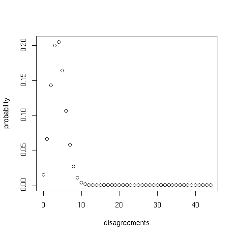
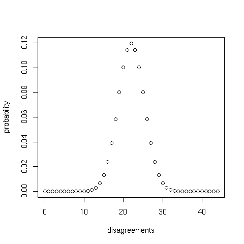
Given n places where two witnesses are defined, any number of disagreements from zero up to and including n is possible. However, the most probable count is the one used to set the probability of disagreement, which in the present context is the number of disagreements in the sample. (In these two examples, the most probable counts are 4 and 22, respectively.) The probabilities of other counts decrease with increasing difference relative to the count used to set the probability of disagreement, tending to produce a bell-shaped curve unless the latter probability is close to zero or one.
In this study, the 95% confidence interval is defined by reference to cumulative probabilities of 0.025 and 0.975. Using the quantile function of the binomial probability function produces 95% confidence intervals of [1, 8] for the first and [16, 28] for the second example. That is, the central 95% of cases can be expected to lie between 1 and 8 counts for the first curve, and between 16 and 28 counts for the second.
| Note |
|---|---|
These intervals were obtained using the quantile function of the
binomial probability distribution, |
The width of the interval changes with the probability of disagreement. In the two examples given above, the width is 8 - 1 = 7 counts for the first example and 28 - 16 = 12 for the second. The following table gives the widths of 95% confidence intervals associated with these and a few other probabilities of disagreement for a sample size of 44:
| p(disagreement) | Interval | Width (counts) |
|---|---|---|
| 0/44 (0) | [0, 0] | 0 |
| 1/44 (0.023) | [0, 3] | 3 |
| 2/44 (0.045) | [0, 5] | 5 |
| 4/44 (0.091) | [1, 8] | 7 |
| 11/44 (0.25) | [6, 17] | 11 |
| 22/44 (0.5) | [16, 28] | 12 |
| 33/44 (0.75) | [27, 38] | 11 |
| 40/44 (0.909) | [36, 43] | 7 |
| 42/44 (0.955) | [39, 44] | 5 |
| 43/44 (0.977) | [41, 44] | 3 |
| 44/44 (1) | [44, 44] | 0 |
As the estimated probability of disagreement (i.e. number of disagreements divided by number of variation units where both witnesses are defined) increases from zero to one half (0.5), the estimated confidence interval width increases as well. The relationship over the range of all probabilities of disagreement from zero to one is symmetrical so that the width associated with a probability p is equal to the width associated with the probability 1 - p. The width varies quite slowly over the central range of probabilities of disagreement, reaching a maximum as the probability approaches one half. (If the sample size is odd then the estimated probability of disagreement cannot equal one half.) All of this is true for every sample size greater than one. To illustrate, the following two tables give the widths of 95% confidence intervals for a range of probabilities of disagreement using sample sizes of 10 and 100:
| p(disagreement) | Interval | Width (counts) |
|---|---|---|
| 1/10 (0.1) | [0, 3] | 3 |
| 2/10 (0.2) | [0, 5] | 5 |
| 5/10 (0.5) | [2, 8] | 6 |
| 8/10 (0.8) | [5, 10] | 5 |
| 9/10 (0.9) | [7, 10] | 3 |
| p(disagreement) | Interval | Width (counts) |
|---|---|---|
| 10/100 (0.1) | [5, 16] | 11 |
| 20/100 (0.2) | [12, 28] | 16 |
| 50/100 (0.5) | [40, 60] | 20 |
| 80/100 (0.8) | [72, 88] | 16 |
| 90/100 (0.9) | [84, 95] | 11 |
The relative width of an interval (i.e. width divided by sample size) decreases as the sample size increases, and the maximum relative width occurs when the probability of disagreement is as close as possible to one half. The following table shows how the maximum relative interval width changes with sample size:
| Sample size | Interval | Maximum relative width |
|---|---|---|
| 2 | [0, 2] | 2/2 (1) |
| 4 | [0, 4] | 4/4 (1) |
| 6 | [1, 5] | 4/6 (0.667) |
| 10 | [2, 8] | 6/10 (0.6) |
| 12 | [3, 9] | 6/12 (0.5) |
| 20 | [6, 14] | 8/20 (0.4) |
| 50 | [18, 32] | 14/50 (0.28) |
| 100 | [40, 60] | 20/100 (0.2) |
| 200 | [86, 114] | 28/200 (0.14) |
| 500 | [228, 272] | 44/500 (0.088) |
| 1000 | [469, 531] | 62/1000 (0.062) |
The relative interval width reaches a maximum as the probability of disagreement approaches one half, and decreases quite slowly as the probability moves away from that value. As a result, using an estimated probability of disagreement as close as possible to one half produces a conservative estimate for the interval width that will be close or equal to the actual value provided that the probability is not too close to zero or one. Every relative interval width estimated in this manner has an associated sample size. To decrease the width it is necessary to increase the sample size. Consequently, a minimum acceptable sample size can be obtained by first specifying a maximum acceptable relative interval width.
Any estimate based on a relative width of one is equivalent to asserting that the estimated value lies somewhere in the range of all possible values, making it worthless. The 95% confidence intervals for a sample size of five are [0, 4] for probability 2/5 and [1,5] for 3/5, making five the smallest sample size that can produce an estimate that is not entirely worthless. For this reason, it is a waste of time to calculate a statistic from the number of agreements or disagreements between two witnesses unless it is based on a sample size of five or more. Narrower relative widths produce more useful statistics. One possibility is to set the maximum acceptable relative width to one half, narrowing the range associated with an estimate to one half of all possible values. If this standard is chosen then the minimum acceptable sample size is twelve.
Given a binomial probability distribution where the probability of a “success” is p and the sample size is n, the mean and standard deviation of the counts of successes and the proportions of successes are as follows ([Moore and McCabe] 1993 380-1). (In the present context, a success is a disagreement between two witnesses at a variation unit where both are defined.)
| Statistic | Formula |
|---|---|
| Mean of counts | np |
| Standard deviation of counts | (np(1 - p))1/2 |
| Mean of proportions | p |
| Standard deviation of proportions | (p(1 - p)/n)1/2 |
As the sample size increases, the normal distribution becomes a better approximation of the binomial one provided that the probability of success is not too close to zero or one. One way to decide whether these conditions are met is to calculate np and n(1 - p). If both are greater than 10, then the normal approximation may be used ([Moore and McCabe] 1993 383).
The central 95% of the normal distribution lies within 1.96 standard deviations of the mean. Consequently, the following formulas give approximate 95% confidence intervals for the number of disagreements and the proportion of disagreements:
| Quantity | Interval |
|---|---|
| Disagreements | d ± 1.96 x (np(1 - p))1/2 |
| Proportion of disagreements | p ± 1.96 x (p(1 - p)/n)1/2 |
Here, n is the number of variation units where two witnesses are both defined, d is the number of disagreements among those n, and p is the estimated proportion of disagreements, which is d/n.
These formulas show how the width of the confidence interval is related to the sample size under the normal approximation. For a count, the width is proportional to the square root of the sample size, while for a proportion it is proportional to the inverse of the square root of the sample size.
The following table compares a few confidence intervals for the number of disagreements obtained using the binomial distribution and its normal approximation where the proportion of disagreement is set at one half:
| Sample size | Binomial interval | Normal approximation |
|---|---|---|
| 6 | [1, 5] | [0.60, 5.40] |
| 10 | [2, 8] | [1.90, 8.10] |
| 20 | [6, 14] | [5.62, 14.4] |
| 50 | [18, 32] | [18.1, 31.9] |
| 100 | [40, 60] | [40.2, 59.8] |
As the maximum interval width occurs when the probability of disagreement is one half, it is possible to use the normal approximation to estimate the minimum sample size required to achieve a desired margin of error ([Moore and McCabe] 1993 582-3):
| Quantity | Estimate | Comment |
|---|---|---|
| Disagreements | n = (2m/1.96)2, or 1.04m2 | m is the maximum acceptable margin of error expressed as a count |
| Proportion of disagreements | n = (1.96/2m)2, or 0.96/m2 | m is the maximum acceptable margin of error expressed as a proportion |
These formulas only apply under conditions where the normal approximation is sufficiently accurate. The conditions given before (np and n(1 - p) greater than 10) correspond to a sample size of 20 when p is one half. Consequently, if one of these formulas returns a sample size of less than 20 then the binomial distribution should be used to obtain a better estimate of the required sample size.
Example 3.2. Confidence level, confidence interval, margin of error, and sample size
In a sample of 44 variation units, two particular witnesses disagree 22 times, corresponding to a simple matching distance of 22/44, or 0.5 units. Using a confidence level of 95% and the binomial probability distribution to approximate the sampling distribution of the number of disagreements between these two witnesses, a 95% confidence interval extending from 16 to 28 disagreements is obtained. This confidence interval can also be expressed in terms of a central estimate and a margin of error that is one half of the interval's width: 22 ± 6 disagreements. The corresponding population parameter is the simple matching distance between these two witnesses that would be obtained if every variation unit were examined. Based on the confidence interval just obtained, the value of this simple matching distance can be asserted to lie between 16/44 and 28/44, or 0.50 ± 0.14 units. If many trials were performed using the same procedure then in 5% of the trials the population parameter would lie outside the confidence interval.
If a maximum margin of error of 0.1 units were desired for the proportion of disagreements then a sample size of approximately 0.96/0.12 or 96 variation units would be required. Even though this estimate is based on the normal approximation, it is reasonably close to what would be obtained with the binomial distribution, which is 100.
The question of whether two witnesses share a statistically significant level of agreement can be answered by way of another question: What range of agreements is expected to occur between two artificial witnesses whose readings have been chosen at random? From a statistical perspective, any number of agreements that falls outside this range is significant.
| Note |
|---|---|
Up until this point, the emphasis has been on counting disagreements in order to calculate a dissimilarity as a proportion of disagreements. Whereas the emphasis is now on agreements rather than disagreements, the statistical arguments apply equally to both. |
A skeptic might say that the level of agreement observed between the readings of two witnesses is the result of random processes rather than a genetic relationship. What would it take to prove beyond reasonable doubt that the skeptic is wrong? One approach is to find the range of agreements that can be expected if the skeptic is right then determine whether observed levels of agreement are significantly different. This method takes a probabilistic view of the evidence and produces a distribution of numbers of agreements expected to occur by chance. Critical values derived from the distribution are then used to decide whether two witnesses have a statistically significant level of agreement.
Textual variations can be arranged as a set of variation units, each containing a set of readings. The probability of occurrence of a particular reading of a particular variation unit is its relative frequency of occurrence among all witnesses:
Here, w(x) is the number of witnesses with reading x, and W is the total number of witnesses where the variation unit is defined.
These quantities are parameters that apply to the entire population of witnesses. In the case of the biblical text, the extant evidence is a mere shadow of the original cloud of witnesses. Consequently, the best one can do is estimate the probability of a reading using sample statistics calculated from a set of extant witnesses. The same formula can then be used to obtain the estimated probability of reading x if w(x) is the number of witnesses in the set with reading x and W is the number of witnesses in the set where the variation unit is defined.
| Note |
|---|---|
Results of analysis based on probabilities calculated from extant witnesses can only be applied to the original population if those witnesses are an unbiased sample of the population. This is probably not the case for the New Testament, where surviving witnesses tend to be late rather than early. Nevertheless, the results do apply to the sample so the quest to establish what constitutes a statistically significant level of agreement among members of the sample remains achievable. Some of the “witnesses” in the given evidence represent groups (e.g. Byz, Lect). Such group witnesses do not affect a test of significance that is based solely upon numbers of agreements. Neither do they confound attempts to recover earlier states of the text in which hypothetical archetypes are constructed at each step of an iterative procedure. It stands to reason that if a group witness were replaced by its constituents then something similar to the group witness itself would be constructed at an early iteration. |
An artificial pseudo-witness can be generated by randomly choosing a reading at each variation unit such that a reading's probability of selection is the same as its relative frequency of occurrence among a sample set of witnesses. By definition, any two of these pseudo-witnesses are unrelated: their readings are the result of random selection, not common ancestry. Lack of relationship does not imply lack of agreement, however. In fact, the probability of agreement between two randomly generated texts at a particular variation unit may be quite high. This probability is calculated by summing the probabilities of combinations of the relevant variation unit's readings that produce agreement. Its method of calculation depends on the chosen method of calculating dissimilarity. Some methods (e.g. simple matching, Euclidean) count both agreements in presence and absence. By contrast, the Jaccard distance only counts agreements in presence. The following equation gives the probability of agreement for the simple matching case:
Equation 3.7. Probability of random agreement (simple matching distance)
For the Jaccard distance, it is the square of the probability of presence of the trait upon which the relevant binary variation unit is based.
Example 3.3. Probability of random agreement (Heb 1.3, simple matching distance)
Among the 24 witnesses that cover all of the variation units of Hebrews recorded in the UBS apparatus, eight support the first reading of Heb 1.3, two support the second, and 14 support the third. As the relative frequencies of occurrence are 8/24, 2/24, and 14/24, the probability of random agreement when using the simple matching distance is (8/24)2 + (2/24)2 + (14/24)2 = 0.458. In this case, which is not atypical, the probability of random agreement is almost 50%.
Once the probability of random agreement among a set of witnesses is known for each variation unit, it is possible to calculate the probability of any number of agreements between two pseudo-witnesses. A distribution of probabilities of random agreement is constructed by plotting the probability of each possible number of agreements from zero up to the number of variation units. Critical values are then obtained from the distribution using a prespecified number called the “alpha” value.
The aim of the exercise is to determine “beyond reasonable doubt” that a particular level of agreement cannot be attributed to chance. Just what is a reasonable level of doubt? Two kinds of error can occur when making a decision based on a statistical analysis of the data: to reject the skeptic's hypothesis when it is true (a “type I” error) or to accept the skeptic's hypothesis when it is false (a “type II” error). The alpha value is the chance of committing a type I error. In contexts where such an error can have grievous consequences, prudence demands a low value of, say, 1%. However, reducing the chance of a type I error increases the chance of a type II error. Consequently, a less stringent value of 5% is commonly employed when the consequences of a type I error are not serious. There is then a one in twenty chance of a type I error.
Critical values are upper and lower bounds on the values of a statistic that may be expected to occur by chance. (In this case, the statistic is the number of agreements.) Given a distribution and an alpha value, critical values are determined by finding the central range of statistic values whose probabilities sum to the complement of the alpha value. Alternatively, the upper (or lower) critical value can be found by summing probabilities in the upper (or lower) tail of the distribution until the sum exceeds one half of the alpha value (0.025). These critical values bracket values of the statistic that can be expected to occur in 95% of cases. Conversely, values of the statistic can be expected to fall outside the range in only 5% of cases. It is therefore reasonably safe to assume that a value outside the range defined by the critical values is not due to chance.
In the present context, calculation of critical values relies on computing the probabilities of a range of numbers of agreements. Three techniques for obtaining critical values are presented below. The first makes a number of assumptions about probabilities of readings so that the binomial distribution can be employed. The second makes an exact calculation based on reading probabilities. Unfortunately, this procedure is so demanding that it can only be used with small numbers of variation units. The third technique employs a “Monte Carlo” calculation that can cope with large numbers of variation units. Its results are not as definitive as the exact calculation but should be better than those of the binomial calculation.
Rather than cover every possible way of measuring agreement, the computer scripts used to demonstrate the binomial and exact techniques employ the simple matching distance alone. The script associated with the Monte Carlo technique is more general and can be used to estimate critical values of dissimilarity using either the simple matching, Jaccard, or Euclidean distance. All of the techniques produce results that are based on probabilities of random agreement among only those witnesses which cover all of the variation units of a specified reference witness.
The first technique uses the binomial distribution to estimate critical values. In so doing, the following assumptions are made concerning the data:
every variation unit has only two readings
the probability of agreement is the same for all variation units
the reading of one variation unit has no effect on the reading of another variation unit.
The first two conditions are not satisfied by the evidence. Only about half of the variation units of the UBS apparatus have but two readings, and it is certain that probabilities of agreement will not be uniform across variation units. The third assumption is probably safe, although it is conceivable that the reading of one variation unit can affect that of another. Despite these violations of the conditions, this technique produces very similar results to the other techniques. It also serves to demonstrate how critical values are derived from a distribution of probabilities of random agreement.
The binomial probability distribution applies to a series of independent trials with only two possible outcomes where the probabilities of both outcomes remain constant throughout. In the present case, the probability of agreement is taken to be the mean value of the probabilities of random agreement calculated from a data matrix. This value is 0.671 when calculated for those witnesses which cover all 44 variation units of the UBS apparatus for Hebrews using the example multistate data matrix and simple matching criterion.
The probability of each number of agreements from zero up to the number of variation units (n) is given by the binomial probability density function. As may be expected, numbers of agreements which are close either to zero or n are relatively rare while numbers of agreements in the central range are relatively common. For an alpha value of 0.05, the critical values are the numbers of agreements at which the cumulative probability first exceeds 0.025 (lower value) and 0.975 (upper value).
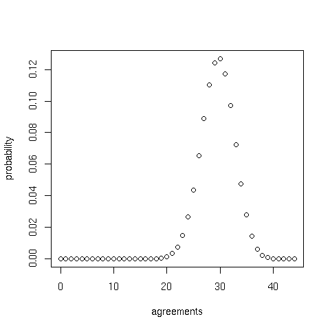
The R script named
binomial.r
estimates critical values using the binomial distribution. In
this case it returns values of 23 (lower) and 35 (upper). That is, 23
or less and 35 or more agreements constitute a statistically
significant level of agreement for two witnesses that are defined in
all 44 variation units of the example multistate data matrix. The
corresponding upper and lower critical values of dissimilarity are 1 -
23/44 = 0.477 and 1 - 35/44 = 0.205 units.
Critical values can be obtained by way of an exact calculation. First, a probability of random agreement is calculated for each variation unit. A probability is then obtained for each possible number of agreements, from a minimum of zero to a maximum equal to the number of variation units.
Each probability of x agreements in n variation units is calculated as follows:
Choose x variation units from the total of n.
Calculate the product of probabilities of random agreement for these x variation units.
Calculate the product of probabilities of random disagreement for the (n - x) remaining variation units, where p(disagreement) = 1 - p(agreement).
Calculate the product of the products obtained in steps 2 and 3. This is the probability of x agreements and (n - x) disagreements for this particular permutation of x variation units.
Sum the probabilities obtained at step 4 for every permutation of x variation units chosen from n variation units.
The weakness of this technique is the large number of calculations required to obtain a result. For example, there are about 2,104,099,000,000 ways to choose 22 variation units from 44, meaning that this many products of 44 probabilities would have to be calculated and summed to obtain the probability of 22 out of 44 agreements. In addition, 43 other calculations of the same kind would be required to complete the distribution, although each would involve fewer permutations.
In practice, it is not necessary to obtain the whole distribution in order to calculate critical values. Instead, the calculation can begin at one end of the distribution and move towards the centre until the cumulative probability reaches one half of the alpha value. The process is then repeated, starting at the other end.
The script
exact.r
obtains critical values by an exact calculation. Execution
time increases rapidly with the number of variation units. My computer
takes about a second to perform the calculation using P13, which has
thirteen variation units, as the reference witness. The calculation
for Codex Vaticanus (B), with 23 variation units, takes about twelve
minutes. A calculation involving all 44 variation units of the example
multistate data matrix would take months to execute.
As the name implies, a Monte Carlo calculation has similarities to a game of chance. At its heart lies a random number generator that acts like a roulette wheel, producing one of a range of possible outcomes. In the present case, each trial produces a set of n numerals, where n is the number of variation units. The random number generator is constrained such that the probability of producing a particular numeral is equal to the relative frequency of the corresponding reading or trait among a set of witnesses. The dissimilarity between this “text” and another one produced in the same way is then calculated using a selected distance measure and stored in an array. Once a preset number of trials has been performed, the array of dissimilarities is sorted into ascending order and the critical values are obtained by referencing particular elements. For example, given an alpha value of 0.05 and 10,000 trials, the upper (or lower) critical value of dissimilarity is found in the 9750th (or 250th) cell of the sorted array.
Due to the stochastic nature of this technique, it is possible for the same input parameters to produce a different pair of critical values from one calculation to the next. Increasing the number of trials makes this less likely to happen but never eliminates the possibility and increases the time required for the calculation as well. I find that using ten thousand trials produces reasonably consistent results in an acceptable time. If successive calculations produce differing pairs of values then the best pair to use is the one produced most often.
The
montecarlo.r
script estimates critical values using a Monte Carlo
calculation. The user supplies an input data matrix, reference
witness, dissimilarity coefficient, alpha value, and number of trials.
If the data matrix is binary then it is appropriate to use the simple
matching, Jaccard, or Euclidean distance as a dissimilarity
coefficient. Only the simple matching distance should be used with a
multistate data matrix.
The following table presents upper and lower critical values of the simple matching distance obtained by these techniques with the example multistate data matrix and UBS, P13, and Codex Vaticanus (B) as reference witnesses. No attempt was made to obtain exact critical values for the 44 variation units covered by the UBS apparatus of Hebrews as the calculation would take a very long time to execute.
| UBS (44 var. units) | P13 (13 var. units) | B (23 var. units) | ||||
|---|---|---|---|---|---|---|
| Lower | Upper | Lower | Upper | Lower | Upper | |
| Binomial | 0.205 | 0.477 | 0.077 | 0.615 | 0.130 | 0.522 |
| Exact | NA | NA | 0.154 | 0.538 | 0.174 | 0.522 |
| Monte Carlo | 0.205 | 0.455 | 0.154 | 0.538 | 0.174 | 0.522 |
The exact and Monte Carlo results agree where both are present. Critical values estimated by the binomial technique are comparable to those of the other techniques. In cases where the number of variation units makes an exact calculation impractical, a Monte Carlo estimate is preferable to a binomial one provided that it is based on enough trials.
Dissimilarities that lie outside the interval defined by the upper and lower critical values are statistically significant because they are not likely to occur through random processes alone. This does not mean that it is impossible for the dissimilarity of a pair of randomly generated pseudo-witnesses to fall outside the critical interval. In fact, the probability that such a dissimilarity will do so is equal to the alpha value used to obtain the critical values, which in the present case is 0.05.
Dissimilarities that lie within the critical interval are not statistically significant. Whereas two witnesses with a dissimilarity in this range may be genetically related, from a statistical perspective their dissimilarity is indistinguishable from that of two pseudo-witnesses constructed from randomly selected readings.
Once critical values are obtained for a particular set of witnesses, the corresponding dissimilarity matrix can be inspected to identify witnesses that fall into the following categories:
witnesses with dissimilarities less than the lower critical value
witnesses with dissimilarities within the interval defined by the upper and lower critical values
witnesses with dissimilarities greater than the upper critical value.
| Note |
|---|---|
This procedure is only valid for a dissimilarity matrix constructed using the exclusive strategy with the same reference witness used to obtain the critical values. |
Witnesses in the first category have dissimilarities that are less than would be expected to occur through random processes alone. This is not to say that they form a group of closely related witnesses. After all, given a large enough sample size, two witnesses with quite large dissimilarities can still belong to this category. Witnesses in the second category do not share a significant level of agreement. Those in the third category form an interesting yet seldom discussed class: witnesses with dissimilarities that are larger than would be expected to occur by chance. Two witnesses with such a large dissimilarity would not be expected to be so different if only random processes had been at work. This class of witnesses may constitute evidence of tendentious editorial practices among ancient copyists.
A chi-squared test compares observed and expected distributions of a statistic to determine the probability that both distributions are from a single population. Taking the number of agreements between two witnesses as the statistic, the distribution of agreements observed among witnesses represented in a data matrix can be compared with the distribution of random agreements obtained with one of the above techniques. A chi-squared test to compare these distributions then determines the probability that the skeptic's hypothesis is true.
The
chisq.r
script performs a chi-squared test based on an input data matrix
and reference witness specified by the user. It uses the simple matching
criterion as a basis for calculating the distribution of random
agreements expected among those witnesses that cover all of the
variation units of the reference witness. If there are less than 25
variation units then an exact calculation is made. Otherwise, the
expected distribution is obtained by a Monte Carlo calculation. The
script produces a plot of the observed and expected distributions of
agreements along with the results of a chi-squared test of the two. The
plot includes a binomial distribution which is purely for reference; it
does not affect the chi-squared calculation. Both the expected and
binomial distributions are normalised to the sum of observed
frequencies.
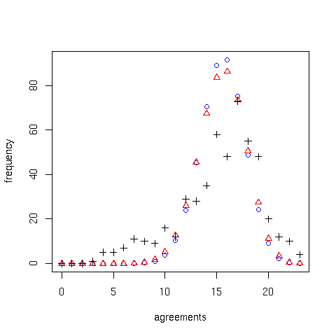
The above plot was produced using the multistate data matrix with Codex Vaticanus (B) as the reference witness. The readings of this codex are recorded for 23 of the variation units present in the UBS apparatus of Hebrews, so the script made an exact calculation of the expected distribution (blue circles). The observed distribution (black crosses) peaks to the right of the expected distribution and has a greater spread. The binomial distribution (red triangles) has a slightly larger spread than the expected distribution but is nevertheless a good approximation.
A chi-squared test of the observed (black crosses) and expected (blue circles) distributions produces an extremely small probability value which indicates that the two are significantly different. It follows that the levels of agreement observed among the witnesses under examination are not consistent with the skeptic's hypothesis. Nevertheless, the similarity of the observed and expected distributions should not be overlooked. A skeptic would be wrong to say that all agreements among the witnesses are due to random processes but may be right to believe that effectively random processes are partially responsible for the observed distribution of levels of agreement.
Table of Contents
This chapter introduces a number of analytical techniques that can be used to explore multivariate data.
Insights into the relative dispositions of extant witnesses can be
gained by arranging them according to their distances from selected
reference witnesses. Two scripts are provided for this purpose. One, which
is named
order-excl.r
, uses the exclusive strategy to eliminate missing data. This
script includes an option to omit witnesses with dissimilarities in the
interval bounded by upper and lower critical values calculated by the
Monte Carlo technique. If the option to omit these witnesses is selected
then the script separates ordered witnesses into two categories:
“Like”: Witnesses with dissimilarities less than the lower critical value.
“Unlike”: Witnesses with dissimilarities greater than the upper critical value.
If the option to omit witnesses in the central interval is not selected then the script outputs the entire list of witnesses in ascending order of distance from the reference witness.
A second script named
order-incl.r
uses the inclusive strategy to ensure that every dissimilarity is
based on a minimum number of variation units. Whereas this allows more
witnesses to be retained, the number of variation units employed to
calculate a dissimilarity can vary from one pair of witnesses to another.
Under these circumstances, no single pair of critical values is applicable
to all dissimilarities. For this reason, order-incl.r does
not have the facility to omit witnesses with dissimilarities between
critical limits.
The following table provides lists of witnesses ordered by dissimilarity relative to a number of reference witnesses. It was made using the multistate data matrix for Hebrews, the simple matching distance, and the inclusive strategy with a minimum of 12 variation units:
| Reference witness | Nearest to farthest witnesses |
|---|---|
| UBS | M33, A, arm, vg-st, M81, cop-sa, vg-cl, vg-ww, U1, B, P46, geo-1, M2464, K, M1739, C, U44, it-comp, geo-2, U150, M1241, M1912, L, it-ar, it-b, syr-p, syr-h, Byz, cop-bo, M424, M436, M1852, M1881, M1962, M2127, U75, D, P, M1319, M2200, slav, M6, M256, M1573, Chrysostom, Lect, it-d, eth-TH, M263, M365, eth-pp, M104, M459 |
| P13 | M424, P46, K, M33, M1852, M1912, M1962, Byz, Lect, slav, UBS, A, L, U44, M6, M81, M365, M436, M2127, arm, Chrysostom, it-b, P, U150, M256, M263, M1241, M1319, M1573, M1881, U1, D, M104, M459, M1739, it-comp, it-d |
| P46 | B, UBS, M1739, M33, cop-sa, it-d, U1, U44, D, M6, arm, M1241, M1881, L, eth-pp, eth-TH, syr-p, geo-1, vg-st, cop-bo, A, K, U75, geo-2, syr-h, vg-ww, M1852, Lect, it-b, it-comp, U150, M81, M424, Byz, it-ar, U243, M256, M1319, M1962, M2127, vg-cl, M263, M436, M1573, M2200, Chrysostom, C, P, M104, M365, M1912, M2464, slav, M459 |
| U1 | M33, A, vg-ww, UBS, M81, cop-bo, it-comp, M2464, vg-st, C, arm, it-b, vg-cl, M436, M2127, L, geo-2, P, M256, M1573, M1881, cop-sa, it-ar, K, M424, geo-1, Byz, slav, syr-p, U75, D, M263, M1241, M1912, M1962, Lect, syr-h, U44, M459, M1739, M1852, it-d, eth-pp, U150, M104, P46, Chrysostom, eth-TH, M365, M2200, B, M1319, M6 |
| A | C, arm, M1912, M33, M2464, UBS, M81, it-ar, P, M436, M2127, U1, M263, M1962, U75, syr-h, vg-st, U150, M256, M424, M1573, syr-p, slav, it-b, vg-cl, vg-ww, K, M104, M365, M459, M1739, cop-bo, Byz, it-comp, M1319, M1852, M1881, Lect, M2200, M6, geo-1, geo-2, cop-sa, Chrysostom, M1241, U44, L, eth-TH, eth-pp, D, it-d, B, P46 |
| B | P46, UBS, M33, arm, syr-p, cop-sa, L, U75, U150, M1241, Lect, syr-h, Byz, geo-2, M6, U1, A, K, M424, M1739, M1881, it-d, eth-pp, eth-TH, U44, D, M1852, M1962, M2200, geo-1, cop-bo, P, M256, M263, M1573, M2127, vg-st, M81, M436, M1319, M2464, it-b, slav, Chrysostom, vg-ww, M1912, it-ar, it-comp, M104, M365, M459, vg-cl |
| C | A, M81, P, M436, M1912, slav, U150, M263, syr-h, M33, arm, it-ar, it-b, M256, M1573, M1962, M2127, vg-ww, vg-st, it-comp, M104, M424, M459, M2200, Byz, Lect, syr-p, Chrysostom, M6, cop-sa, M365, M1319, M1852, M1881, geo-2, eth-pp, eth-TH, vg-cl, UBS, U1, cop-bo, K, M1241, M1739, L, U44, geo-1, D, it-d, P46 |
| D | it-d, U44, vg-cl, vg-ww, geo-1, syr-h, vg-st, M1319, syr-p, slav, UBS, K, M365, M1852, M1912, it-comp, L, M6, U1, A, P, it-ar, M256, M1241, M1573, M1739, M1962, M2127, M2464, cop-bo, M33, arm, Chrysostom, Byz, Lect, M104, M263, M459, geo-2, C, U75, eth-TH, U150, M81, M424, M436, P46, it-b, M2200, M1881, eth-pp, cop-sa, B |
| D-2 | Byz, M1852, Lect, L, M2200, K, M424, M1962, Chrysostom, M1881, M365, M1241, geo-2, slav, U150, M263, M436, M459, M6, M104, M256, M1319, M1573, M2127, eth-pp, M1912, eth-TH, syr-h, geo-1, U44, arm, cop-bo, P, M33, M81, it-b, A, M1739, it-ar, cop-sa, UBS, U1, P46, it-comp, it-d, D |
| K | L, Byz, M1852, Lect, M424, M2200, M1241, M1319, geo-2, Chrysostom, slav, M1881, M1962, M365, M1912, M256, U75, U150, M263, M1573, M2127, syr-h, eth-TH, geo-1, U44, M6, M33, eth-pp, cop-bo, P, M436, M459, syr-p, vg-cl, vg-st, A, M104, it-ar, M2464, UBS, M1739, vg-ww, it-b, M81, arm, C, it-comp, cop-sa, U1, D, it-d, B, P46 |
| L | Byz, K, M1852, M1241, Lect, M2200, M424, Chrysostom, M1319, M1881, M1962, syr-h, geo-2, slav, M256, U44, M6, U150, M263, M1573, M2127, M33, M365, M459, U75, vg-st, M104, M1912, eth-pp, geo-1, P, M436, vg-ww, it-ar, eth-TH, M2464, vg-cl, it-b, UBS, M81, cop-bo, syr-p, U1, A, M1739, arm, cop-sa, D, it-comp, B, it-d, P46 |
| P | M2464, M1912, C, M263, M436, M459, M104, M1319, M1962, slav, M81, M256, M365, M2127, syr-h, M2200, eth-TH, U44, A, U150, M424, M1573, M33, eth-pp, Byz, U75, vg-cl, K, M1852, Lect, Chrysostom, vg-st, L, it-ar, arm, M6, M1241, M1881, vg-ww, cop-bo, syr-p, geo-2, it-b, geo-1, it-comp, U1, cop-sa, UBS, D, M1739, it-d, B, P46 |
| U44 | M2464, L, M6, P, U150, M365, M1962, syr-h, geo-1, K, M436, M1319, M1852, M1912, Lect, Chrysostom, vg-st, slav, M81, M256, M263, M1881, M2127, Byz, U75, M2200, vg-cl, vg-ww, eth-pp, eth-TH, geo-2, UBS, D, M104, M424, M1241, M1573, it-ar, M33, U243, syr-p, A, M459, cop-bo, arm, C, it-b, M1739, it-d, U1, it-comp, P46, cop-sa |
| U75 | Byz, M1962, Lect, K, M256, M263, M365, M424, M1319, M1852, M2127, A, L, P, M104, M459, M1241, M1573, M1881, M2200, arm, M6, syr-h, M436, M1912, U44, slav, U150, M33, M2464, syr-p, eth-TH, geo-2, Chrysostom, M81, M1739, vg-st, eth-pp, it-ar, UBS, vg-cl, vg-ww, cop-bo, geo-1, U1, it-b, B, D, it-comp, it-d, P46, cop-sa |
| U150 | M2464, syr-h, C, M1962, Byz, vg-st, M263, M1852, M2127, M2200, Chrysostom, L, U44, K, P, M256, M436, M1319, M1573, M1912, vg-cl, vg-ww, arm, eth-pp, M81, M424, M1241, Lect, slav, M33, eth-TH, A, M365, M1881, M6, geo-1, M104, M459, it-ar, syr-p, it-b, geo-2, cop-sa, U75, UBS, cop-bo, M1739, it-comp, B, U1, D, it-d, P46 |
| U243 | M1739, M1881, M81, M6, M365, M436, M1912, M1962, eth-pp, eth-TH, slav, U150, M104, M256, M263, M424, M459, M1852, M2127, M33, Byz, it-ar, Lect, syr-p, A, K, P, M1573, M2200, cop-bo, geo-1, Chrysostom, it-b, syr-h, M1241, M1319, geo-2, arm, U44, cop-sa, it-comp, UBS, U1, D, it-d, P46 |
| M6 | M1881, Lect, U243, M1739, M1962, M2127, syr-h, M424, M2200, Byz, M256, M263, M1573, M1912, Chrysostom, L, vg-st, U44, M365, M1241, M1319, M1852, it-ar, geo-1, K, M436, eth-pp, eth-TH, vg-cl, vg-ww, syr-p, U75, C, U150, M104, M459, cop-bo, it-b, slav, geo-2, P, M81, M33, arm, A, cop-sa, it-comp, M2464, UBS, D, it-d, P46, B, U1 |
| M33 | M81, U1, A, M2464, C, arm, vg-st, cop-sa, UBS, M2127, vg-ww, syr-h, Byz, P, M424, L, cop-bo, it-b, K, U150, M256, M436, M1573, M1912, M1962, Lect, it-ar, it-comp, M1241, M1881, M2200, geo-2, vg-cl, syr-p, M263, M1852, slav, Chrysostom, M6, U75, geo-1, M1739, eth-pp, U44, M104, M459, eth-TH, M1319, M365, B, P46, D, it-d |
| M81 | M2464, C, M436, vg-st, M33, M1912, vg-ww, slav, cop-bo, it-b, it-ar, A, P, M1962, arm, M104, M459, M2127, vg-cl, U150, M365, M1881, Chrysostom, cop-sa, it-comp, UBS, M256, M263, M424, M1573, M1852, U44, syr-h, geo-1, U1, Byz, M6, M2200, geo-2, M1241, M1319, Lect, K, M1739, L, U75, syr-p, eth-pp, eth-TH, D, it-d, P46, B |
| M104 | M459, M256, M263, M436, M2464, M1573, M1912, M2127, M365, Lect, slav, M424, M1962, M2200, Byz, P, M1319, M1852, Chrysostom, M1241, M81, syr-h, C, cop-bo, M1881, U75, arm, L, it-ar, M6, A, K, U150, it-b, geo-2, cop-sa, eth-pp, U44, eth-TH, vg-cl, vg-st, M33, geo-1, syr-p, vg-ww, it-comp, M1739, U1, D, UBS, it-d, P46, B |
| M256 | M1573, M2127, M263, M104, M459, Lect, Byz, M2464, M436, syr-h, M424, M1319, M1912, M2200, M365, M1241, cop-bo, L, M6, C, slav, K, P, M1881, M1962, arm, eth-pp, it-b, U75, U150, M1852, Chrysostom, eth-TH, it-ar, M33, vg-st, geo-2, A, M81, U44, cop-sa, vg-ww, syr-p, it-comp, vg-cl, geo-1, M1739, U1, UBS, D, it-d, B, P46 |
| M263 | M256, M1573, M2127, M459, Lect, M104, M436, M1319, Byz, M2464, syr-h, C, P, M365, M1912, slav, M424, M1241, M1881, M1962, eth-pp, M6, U150, M1852, M2200, arm, cop-bo, L, eth-TH, geo-2, U75, K, A, Chrysostom, M81, it-ar, U44, cop-sa, it-b, syr-p, M33, geo-1, vg-st, M1739, vg-cl, vg-ww, it-comp, U1, UBS, D, it-d, B, P46 |
| M365 | M436, M1912, M2464, M459, M1962, slav, M104, M263, M424, M1319, M1852, M2127, M2200, K, M256, Byz, Lect, P, M1573, Chrysostom, U75, U44, M6, L, eth-TH, M81, M1881, vg-cl, vg-st, eth-pp, U150, M1241, it-ar, arm, C, syr-h, vg-ww, A, cop-bo, geo-2, geo-1, it-b, it-comp, syr-p, cop-sa, M1739, M33, D, UBS, it-d, U1, P46, B |
| M424 | Byz, M2200, M1852, M1962, Lect, L, K, slav, M1241, M1912, M459, M2127, Chrysostom, M104, M256, M365, M436, M1319, M6, geo-2, M263, M1573, M1881, syr-h, U75, it-ar, P, M33, C, M2464, cop-bo, U150, vg-st, eth-pp, A, M81, arm, cop-sa, geo-1, vg-ww, eth-TH, syr-p, it-b, vg-cl, U44, it-comp, M1739, UBS, U1, it-d, D, B, P46 |
| M436 | M2464, M1912, M365, M459, M81, M104, slav, M263, M1962, M2127, C, arm, M256, P, M424, M1573, Lect, M1319, M1852, M2200, Byz, A, U150, M1881, vg-st, U44, M6, M33, Chrysostom, vg-ww, it-b, cop-bo, K, M1241, it-ar, syr-h, cop-sa, U75, geo-2, vg-cl, L, geo-1, eth-pp, it-comp, eth-TH, U1, UBS, M1739, syr-p, D, it-d, B, P46 |
| M459 | M104, M263, M436, M256, M2464, M365, M1573, M1912, M2127, Lect, slav, M424, M1962, Byz, P, M1319, M1852, M2200, M1241, Chrysostom, M81, M1881, syr-h, C, L, cop-bo, U75, arm, K, it-ar, M6, geo-2, eth-pp, A, U150, it-b, cop-sa, eth-TH, vg-cl, vg-st, M33, geo-1, syr-p, U44, vg-ww, it-comp, M1739, U1, D, UBS, it-d, P46, B |
| M1175 | M424, M1852, Byz, Lect, L, M2200, K, M1962, slav, M365, M436, M459, M1241, M104, M263, M1881, M1912, Chrysostom, syr-p, geo-2, eth-pp, eth-TH, A, P, M81, M256, M1319, M33, U150, M1573, M2127, syr-h, M6, cop-sa, UBS, U44, geo-1, cop-bo, arm, vg-st, U1, it-ar, vg-ww, M1739, it-b, D, it-comp, vg-cl, P46, it-d |
| M1241 | L, Byz, Lect, M1852, K, M424, M1319, syr-h, M256, M263, M459, M1881, M1962, M2200, geo-2, slav, M104, M1573, M2127, Chrysostom, M6, U150, U75, M365, M436, M1912, it-ar, M33, cop-sa, vg-st, syr-p, arm, M2464, P, M81, eth-pp, vg-cl, vg-ww, cop-bo, U44, it-b, UBS, eth-TH, geo-1, A, M1739, C, it-comp, U1, D, B, it-d, P46 |
| M1319 | M1852, Byz, Lect, K, M263, M1241, L, slav, M256, M365, M424, M459, M1912, syr-h, P, M104, M1573, M2127, M2200, Chrysostom, M436, M1962, geo-2, U75, M6, it-ar, U150, U44, vg-cl, M2464, C, vg-st, eth-TH, M1881, arm, geo-1, A, M81, eth-pp, vg-ww, cop-bo, it-b, it-comp, syr-p, M33, D, cop-sa, UBS, M1739, it-d, U1, P46, B |
| M1573 | M256, M2127, M263, M104, M459, Lect, syr-h, Byz, M436, M1912, M2464, M424, M1319, M2200, cop-bo, M6, C, M365, M1241, arm, L, it-b, slav, K, P, U150, M1881, M1962, Chrysostom, eth-pp, M1852, it-ar, U75, M33, vg-st, eth-TH, A, M81, cop-sa, geo-2, vg-ww, syr-p, U44, it-comp, vg-cl, geo-1, M1739, U1, UBS, D, it-d, B, P46 |
| M1739 | M1881, M6, A, UBS, K, M1962, M2127, vg-cl, vg-st, M33, syr-p, geo-1, M81, M1852, M1912, Byz, Lect, it-ar, vg-ww, cop-bo, U75, M256, M263, M424, M1241, M1573, C, syr-h, L, arm, Chrysostom, M2200, P46, it-b, geo-2, M365, eth-TH, U150, M104, M436, M459, M1319, it-comp, it-d, eth-pp, U44, cop-sa, U1, D, P, M2464, slav, B |
| M1852 | Byz, L, K, M424, Lect, M2200, M1962, Chrysostom, slav, M1241, M1319, M1881, M365, M459, M1912, geo-2, M104, U150, M263, M436, U75, M6, M256, syr-h, M2464, geo-1, M1573, M2127, U44, vg-st, P, M81, it-ar, C, vg-ww, cop-bo, M33, A, eth-pp, vg-cl, arm, syr-p, M1739, eth-TH, it-b, cop-sa, UBS, D, it-comp, U1, it-d, B, P46 |
| M1881 | M6, Byz, Lect, M1739, M1852, M1962, L, K, M263, M424, M1241, M256, M2127, M2200, Chrysostom, cop-bo, M436, M459, M1573, geo-2, M81, M104, M365, M1912, slav, U75, U150, M2464, U44, M33, C, syr-h, geo-1, vg-st, eth-pp, M1319, syr-p, it-b, A, P, eth-TH, vg-ww, it-ar, cop-sa, vg-cl, arm, UBS, U1, it-comp, B, D, P46, it-d |
| M1912 | M436, slav, M2464, M365, P, M104, M424, M459, M1962, M2127, C, M2200, M81, A, M256, M263, M1319, M1573, M1852, arm, Chrysostom, Byz, K, M6, Lect, it-ar, cop-bo, U150, vg-cl, vg-st, syr-h, it-b, syr-p, eth-TH, geo-2, M1881, U44, M33, cop-sa, vg-ww, it-comp, geo-1, L, eth-pp, M1241, U75, UBS, M1739, D, U1, it-d, B, P46 |
| M1962 | M424, M1852, Byz, M2200, Lect, slav, M365, M436, M1912, M2464, M459, M1881, M6, L, Chrysostom, K, U150, M104, vg-st, P, M263, M1241, M2127, U75, C, vg-ww, M81, M256, M1319, geo-1, U44, M1573, vg-cl, syr-h, arm, geo-2, A, it-ar, M33, eth-pp, cop-bo, eth-TH, cop-sa, M1739, syr-p, it-b, it-comp, UBS, U1, D, it-d, B, P46 |
| M2127 | M256, M1573, M263, M104, M436, M459, M1912, syr-h, Lect, M2464, M424, M6, Byz, M365, M2200, cop-bo, arm, it-b, M1319, M1962, C, it-ar, vg-st, P, U150, M1241, M1881, M33, L, eth-pp, U75, slav, A, K, M81, vg-ww, Chrysostom, eth-TH, M1852, cop-sa, geo-2, syr-p, U44, it-comp, vg-cl, M1739, geo-1, U1, UBS, D, it-d, B, P46 |
| M2200 | M424, Byz, M1852, Chrysostom, L, M1962, Lect, K, slav, M1912, M104, M256, M365, M459, M2127, M6, vg-st, it-ar, M1241, M1319, M1573, vg-ww, syr-h, M2464, P, U150, M263, M436, M1881, eth-pp, vg-cl, C, eth-TH, U75, geo-2, it-b, M33, U44, M81, geo-1, it-comp, cop-bo, A, arm, cop-sa, syr-p, M1739, UBS, it-d, U1, D, B, P46 |
| M2464 | M436, M81, M1912, slav, P, M104, M365, M459, arm, vg-st, U150, M256, M263, M1962, M2127, vg-ww, A, M33, M1573, U44, it-ar, it-b, M2200, cop-sa, Chrysostom, cop-bo, M424, M1852, vg-cl, geo-1, syr-h, it-comp, M1319, M1881, Byz, eth-pp, Lect, UBS, U1, K, L, M1241, U75, eth-TH, geo-2, M6, syr-p, D, M1739, it-d, B, P46 |
| Byz | M1852, Lect, L, M424, M2200, K, M1241, M1962, Chrysostom, slav, M1319, M256, M263, M1881, geo-2, M459, M1573, M2127, U75, M104, M1912, M6, syr-h, U150, M365, M436, M33, C, eth-pp, P, it-ar, vg-st, eth-TH, cop-bo, U44, geo-1, M2464, it-b, vg-ww, A, M81, arm, vg-cl, syr-p, M1739, UBS, cop-sa, it-comp, U1, D, B, it-d, P46 |
| Lect | Byz, L, M424, M1852, M263, M1241, M2200, K, M6, M256, M1319, M1962, slav, M459, M1573, M1881, M2127, Chrysostom, geo-2, M104, syr-h, M365, M436, M1912, U75, cop-bo, eth-pp, U150, U44, M33, eth-TH, P, it-ar, arm, geo-1, syr-p, M2464, it-b, cop-sa, A, M81, vg-st, M1739, vg-ww, vg-cl, it-comp, UBS, U1, D, B, it-d, P46 |
| it-ar | vg-st, vg-ww, it-b, it-comp, vg-cl, M2200, C, cop-bo, Chrysostom, M2464, slav, M81, M1912, M2127, syr-h, A, M424, M1319, M6, geo-1, M256, M1573, M1962, Byz, M33, eth-pp, M104, M263, M365, M436, M459, M1241, M1852, Lect, L, eth-TH, K, P, U150, cop-sa, geo-2, M1881, arm, it-d, U44, UBS, M1739, syr-p, U75, U1, D, P46, B |
| it-b | it-ar, it-comp, vg-st, vg-ww, cop-bo, M2127, vg-cl, C, M2464, M81, M256, M1573, M1912, M33, Chrysostom, M436, M2200, geo-1, slav, eth-pp, A, M263, M6, Byz, geo-2, U150, M104, M424, M459, M1881, eth-TH, syr-p, Lect, arm, syr-h, cop-sa, U1, K, M1241, M1319, M1962, L, UBS, P, M365, M1852, it-d, M1739, U44, U75, D, P46, B |
| it-comp | vg-cl, vg-ww, it-b, it-ar, vg-st, cop-bo, C, M81, M1912, M2464, cop-sa, M33, it-d, M2127, Chrysostom, U1, A, M2200, geo-1, slav, UBS, M256, M436, M1319, M1573, M6, M365, M424, eth-TH, arm, syr-p, K, P, M104, M459, M1962, eth-pp, Byz, D, U150, M263, M1241, M1739, M1852, syr-h, geo-2, Lect, L, M1881, U44, U75, P46, B |
| it-d | vg-cl, D, vg-ww, it-comp, vg-st, it-ar, geo-1, eth-TH, it-b, cop-bo, eth-pp, M1739, U44, M6, UBS, K, M1319, syr-h, syr-p, Chrysostom, U1, M365, M1912, M1962, M2127, P46, geo-2, M2200, L, A, M256, M424, M1852, arm, M33, cop-sa, Byz, P, U150, M1241, M1573, M2464, slav, C, Lect, M81, M263, M1881, B, U75, M104, M436, M459 |
| it-v | A, P, U44, U75, U150, M33, M81, M436, M1962, M2464, arm, M256, M263, M365, M1881, M1912, M2127, it-ar, syr-h, slav, K, L, M6, M104, M424, M459, M1241, M1573, M1852, M2200, Byz, it-b, syr-p, eth-pp, eth-TH, geo-1, Chrysostom, UBS, U243, M1319, it-comp, geo-2, U1, B, D, M1739, it-d, P46 |
| it-z | it-b, cop-bo, it-comp, it-ar, it-d, M81, M1739, M2127, M6, Byz, U1, A, M256, M424, M1319, M1573, M1881, M1912, M1962, Chrysostom, Lect, geo-1, geo-2, slav, UBS, M263, M436, M1852, U44, M33, K, P, U150, M104, M459, M1241, arm, syr-h, cop-sa, P46, M365, D |
| vg-cl | vg-ww, it-comp, vg-st, it-ar, it-b, Chrysostom, geo-1, M2200, U150, M81, M1912, M1962, M2464, it-d, M6, P, M365, M1319, cop-bo, UBS, A, K, M436, M2127, M33, U44, slav, M424, M1241, M1739, M1852, eth-TH, L, Byz, syr-h, U1, D, M104, M256, M459, M1573, M1881, arm, eth-pp, cop-sa, M263, Lect, U75, geo-2, syr-p, P46, B |
| vg-st | vg-ww, it-ar, vg-cl, it-b, it-comp, M2464, M81, Chrysostom, M2200, M1962, M33, geo-1, U150, M2127, cop-bo, M6, eth-pp, slav, M436, M1912, eth-TH, UBS, A, M256, M365, M424, M1573, M1852, arm, L, Byz, syr-h, U44, K, P, M1241, M1319, M1881, cop-sa, it-d, U1, M1739, Lect, M104, M263, M459, U75, geo-2, D, syr-p, P46, B |
| vg-ww | vg-st, vg-cl, it-ar, it-comp, it-b, M81, M2464, Chrysostom, M2200, M1962, cop-bo, M33, geo-1, U150, M2127, slav, eth-pp, M6, M436, M1912, it-d, eth-TH, UBS, U1, A, M256, M365, M424, M1573, M1852, arm, L, Byz, syr-h, cop-sa, U44, K, P, M1241, M1319, M1881, D, M1739, Lect, M104, M263, M459, U75, geo-2, syr-p, P46, B |
| syr-p | syr-h, geo-2, cop-sa, cop-bo, eth-TH, M1912, M6, eth-pp, A, K, M2127, Lect, U150, M33, M256, M263, M424, M1241, M1573, M1881, geo-1, it-b, slav, Byz, P, M1739, M1852, M1962, Chrysostom, U75, U44, L, M2200, UBS, M81, M104, M365, M459, M1319, it-ar, it-comp, arm, D, M2464, vg-st, U1, M436, vg-cl, vg-ww, it-d, P46 |
| syr-h | M2127, L, U150, M256, M263, M1241, M1573, C, M6, Lect, M1319, Chrysostom, syr-p, Byz, slav, M2200, P, M424, geo-2, arm, it-ar, U44, K, M33, M104, M459, M1852, M1912, M1962, M2464, A, vg-st, U75, M81, M365, M436, M1881, geo-1, vg-ww, eth-pp, it-b, cop-sa, vg-cl, eth-TH, UBS, D, M1739, cop-bo, it-comp, U1, it-d, P46 |
| syr-pal | U150, arm, M33, M81, M436, M1852, M1962, syr-h, geo-1, Chrysostom, M2200, UBS, K, L, M424, M1241, M1573, M1881, M1912, M2127, Byz, Lect, geo-2, slav, P46, it-b, syr-p, U75, A, P, M256, M263, M1319, eth-pp, it-ar, M104, M365, M459, M1739, eth-TH, D, it-d, it-comp, U1 |
| cop-sa | cop-bo, M33, M2464, arm, syr-p, M81, M1912, M2127, it-comp, UBS, M256, M263, M424, M436, M1241, M1573, vg-ww, vg-st, it-ar, U150, M104, M459, M1962, Lect, eth-pp, slav, it-b, geo-2, syr-h, A, M1881, M6, M2200, eth-TH, geo-1, Chrysostom, M365, M1852, vg-cl, Byz, L, U1, K, P, M1319, M1739, P46, U44, it-d, D, U75 |
| cop-bo | it-b, cop-sa, M2127, it-comp, it-ar, M81, M256, M1573, vg-ww, vg-st, M263, M1881, M1912, geo-1, M2464, syr-p, M33, M104, M424, M459, Lect, geo-2, K, M436, M1962, Byz, slav, vg-cl, Chrysostom, M6, U1, A, M365, M1852, eth-pp, eth-TH, P, M1241, M1319, M2200, L, U150, M1739, arm, U44, UBS, syr-h, it-d, U75, D, P46 |
| cop-fay | cop-sa, cop-bo, M256, M263, M2127, M1573, A, P, M33, M104, M424, M459, M1912, arm, it-ar, it-b, it-comp, eth-pp, eth-TH, syr-p, Lect, M436, M2464, vg-cl, vg-ww, vg-st, syr-h, slav, U1, M81, M365, M1319, M1881, M1962, M2200, it-d, geo-1, geo-2, UBS, K, U150, M1241, M1739, Byz, P46, Chrysostom, D, L, M1852, U75 |
| arm | M2464, M436, A, M1912, M2127, C, M33, M81, M256, M263, M1573, syr-h, cop-sa, slav, U150, M1962, U75, UBS, M104, M459, vg-st, geo-2, M365, M424, Lect, vg-ww, geo-1, P, M1241, M1319, Byz, M6, it-b, U1, M1852, it-ar, Chrysostom, M2200, vg-cl, K, M1881, cop-bo, L, it-comp, M1739, syr-p, U44, eth-pp, B, eth-TH, D, it-d, P46 |
| eth-pp | eth-TH, M263, M2200, M256, M2127, vg-st, P, U150, M1573, Byz, Lect, slav, M6, vg-ww, syr-p, K, M365, M424, M1912, M1962, it-ar, Chrysostom, L, it-b, M459, M1881, M2464, geo-2, U44, C, M104, M436, M1241, M1319, M1852, syr-h, cop-sa, cop-bo, geo-1, M33, vg-cl, M81, U75, it-comp, it-d, arm, A, M1739, UBS, U1, D, P46, B |
| eth-TH | eth-pp, P, M263, syr-p, K, M256, M365, M1912, M2127, M2200, M6, vg-st, U150, M1573, Byz, Lect, slav, vg-ww, M424, M1319, M1962, it-ar, Chrysostom, L, it-b, U44, C, M459, M1881, cop-bo, vg-cl, geo-2, M2464, U75, M104, M436, M1241, M1852, syr-h, cop-sa, geo-1, it-comp, M33, it-d, A, M81, M1739, arm, UBS, U1, D, P46, B |
| geo-1 | geo-2, vg-st, slav, M1962, Chrysostom, vg-cl, vg-ww, cop-bo, K, U44, M6, M1852, it-ar, M2464, M1912, Byz, Lect, it-b, L, syr-h, U150, M81, M424, M1881, arm, syr-p, UBS, M436, M1319, M2200, M33, eth-pp, it-comp, A, M263, M365, M1739, M2127, cop-sa, eth-TH, D, P, M104, M256, M459, M1241, M1573, it-d, C, U1, U75, P46, B |
| geo-2 | geo-1, slav, K, Byz, Lect, M424, M1852, L, M1241, syr-h, syr-p, M263, M1319, M1881, M1912, M1962, Chrysostom, cop-bo, M256, M2127, M2200, arm, M436, M459, M1573, M33, C, M6, eth-pp, it-b, U150, M81, M104, M365, it-ar, cop-sa, eth-TH, M2464, U44, UBS, A, P, U75, vg-st, U1, M1739, it-comp, vg-cl, vg-ww, it-d, D, B, P46 |
| slav | M1912, M2464, M1852, Chrysostom, Byz, M424, M436, M1962, geo-2, Lect, M2200, M365, M459, U243, C, K, M104, M1319, M81, M263, L, it-ar, geo-1, syr-h, P, M256, M1241, vg-st, M1573, M2127, arm, eth-pp, U150, M1881, vg-ww, eth-TH, U44, cop-bo, A, it-b, M6, M33, vg-cl, syr-p, U75, cop-sa, it-comp, D, UBS, U1, M1739, it-d, B, P46 |
| Chrysostom | M2200, M1852, Byz, slav, L, Lect, K, M424, M1962, vg-st, M1912, syr-h, vg-ww, it-ar, M104, M459, M1319, M6, U150, M365, M1241, M1881, vg-cl, M2464, geo-1, M256, M1573, M2127, geo-2, it-b, C, M81, M263, M436, U44, eth-pp, cop-bo, P, it-comp, eth-TH, M33, syr-p, U75, arm, A, cop-sa, M1739, UBS, it-d, D, U1, B, P46 |
| Cyril | M436, M1912, slav, M2464, P, U150, M81, M1962, M2200, Chrysostom, M104, M365, M424, M459, M1319, M1852, arm, M33, it-ar, cop-sa, K, M256, M1241, M2127, Byz, L, it-b, it-comp, cop-bo, eth-pp, eth-TH, UBS, A, M263, M1573, Lect, geo-1, geo-2, U75, M1881, M6, U1, it-d, D, B, M1739, P46 |
| Theodoret | P, M256, M263, M365, M1319, M2127, A, K, M1573, M1912, arm, eth-TH, U44, UBS, U150, M33, M104, M424, M436, M459, M1241, M1739, eth-pp, geo-2, D, M81, M1852, M1962, it-ar, it-comp, Chrysostom, M1881, P46, U1, it-b, geo-1 |
| Ambrose | M1739, it-d, K, M256, M1573, M1881, M2127, it-b, eth-pp, eth-TH, UBS, L, U150, M263, M424, M1241, it-comp, arm, A, M33, M104, M365, M436, M459, M1319, M1852, M1912, M1962, U1, P, M81, D |
The witnesses are arranged in ascending order of dissimilarity, meaning that the distance from the reference witness increases as one moves from left to right in an ordered list. A group of witnesses within a list may be equidistant from the reference witness. If so, the order of witnesses within that group is arbitrary. As the lists do not include distances, it is necessary to inspect the corresponding dissimilarity matrix in order to identify such groups.
These lists provide insights into the overall structure of what might be called the textual space occupied by extant witnesses. Some witnesses (e.g. P46, B) have a relatively small dissimilarity while others (e.g. P46, M459) have a relatively large one. Each list represents a one-dimensional projection of the multidimensional space that the witnesses occupy, representing a graduated series of dissimilarities with respect to a reference witness. By considering more than one list, it is possible to piece together a mental picture of the textual space, with particular combinations of witnesses tending to be found near each other. However, apart from the most trivial cases, it is difficult to construct a mental image that accurately reflects the actual shape of the space. Fortunately, multivariate analysis techniques exist which are able to extract witness coordinates. They use methods from the field of linear algebra and might therefore intimidate someone who has not mastered the mathematics but still wants to apply the techniques to textual data. I encourage anyone who does feel intimidated to press on regardless. Just as it is not necessary to understand every piece of technology that makes a computer work in order to use one, so it is not necessary to know how to do matrix algebra and eigen-analysis in order to apply the methods which are about to be introduced.
Principal components analysis (PCA) seeks to obtain a set of uncorrelated variables from the variables of a data matrix. The uncorrelated variables, called principal components, are linear combinations of the original variables. They are extracted in order of importance, the first accounting for more variation than the second, the second for more than the third, and so on.
The general hope of principal components analysis is that the first few components will account for a substantial proportion of the variation in the original variables ... and can, consequently, be used to provide a convenient lower-dimensional summary of these variables ([Everitt] 2005 41).
The script named
pca.r
performs principal components analysis on an input data matrix. If
the original data is nominal, as is assumed to be the case throughout this
study, then it must first be transformed into binary form. This is because
the analysis calculates either a covariance or correlation matrix from the
data matrix, and the result of such a calculation is only meaningful for
binary nominal data. Missing data can frustrate the analysis; for example,
two witnesses might have no variation units in common, making it
impossible to calculate the correlation between them. This script uses the
exclusive strategy to eliminate missing data from the data matrix,
dropping columns not present in a specified reference witness then
dropping rows that still contain missing data. The script's output
consists of two items:
a scatter plot matrix that places the witnesses according to their scores on a set of principal components specified by the user; and
a listing of the “proportion of variance” accounted for by each principal component.
The proportion of variance indicates how much of the total variance in the data is explained by a principal component; the larger the proportion of variance, the more important the principal component. The following table reproduces some of the proportion of variance data from the listing obtained with the binary data matrix of Hebrews when the UBS text is used as the reference witness. Cumulative proportions are included as well, with all figures rounded to three decimal places.
| Principal component | Proportion of variance | Cumulative proportion |
|---|---|---|
| 1 | 0.165 | 0.165 |
| 2 | 0.155 | 0.320 |
| 3 | 0.109 | 0.430 |
| 4 | 0.094 | 0.524 |
| 5 | 0.075 | 0.598 |
| 6 | 0.071 | 0.669 |
| 7 | 0.052 | 0.721 |
| 8 | 0.048 | 0.769 |
| 9 | 0.038 | 0.807 |
| 10 | 0.033 | 0.840 |
| ... | ... | ... |
| 20 | 0.005 | 0.994 |
| 21 | 0.003 | 0.997 |
| 22 | 0.003 | 0.999 |
| 23 | 0.001 | 1.000 |
| 24 | 0.000 | 1.000 |
Each cumulative proportion is the sum of proportions up to and including the current one. In this case, the first component accounts for 16.5% of the variation, the second for 15.5%, and so on. Nine components are required to account for 80% of the variation and 23 are required to account for all of it. This shows that the UBS apparatus data has a high dimensionality so more than a few principal components are required to account for the bulk of the variation.
The scatter plot matrix for the first three principal components includes panels for “PC2” vs “PC1” (row 2, column 1), “PC3” vs “PC1” (row 1, column 1), “PC3” vs “PC2” (row 1, column 2) and corresponding panels in which the order of axes is reversed. (Different sets of components can be specified in the script allowing other dimensions to be explored.)
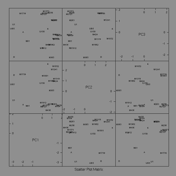
The “PC2” vs “PC1” panel (second row, first column) plots witness scores on the first two principal components. This is a helpful starting place for comprehending the relative positions of witnesses in textual space. Scores on the first principal component (i.e. the horizontal axis) happen to separate texts commonly characterised as “Byzantine” (witnesses on the right) from their non-Byzantine counterparts (witnesses on the left).
The second principal component accounts for almost the same proportion of variance as the first (15.5% as compared with 16.5%). This means that when it comes to variation between witnesses, the difference between witnesses like M436 (bottom) and K (top) is almost as important as the difference between witnesses like U1 (left) and M459 (right).
The third principal component accounts for another 10.9% of the total variation. It enables certain witnesses that appear to be close together in the plot of the first two principal components to be differentiated. To illustrate, the “PC2” vs “PC3” panel (second row, third column) plots witness scores on the second and third principal components. It shows that M1739 and D, which appear to be close together in the “PC2” vs “PC1” panel, are actually quite far apart. An analogous situation occurs when two stars that are separated by a great distance appear to be close together because they lie in approximately the same direction from our perspective.
Principal component scores are an optimal means of characterising a witness. When it comes to explaining variance, they are at least as efficient as ad hoc indices such as percentage of “Byzantine” readings or percentage of “Alexandrian” readings. Despite their efficiency, the high dimensionality of the data means that numerous principal components are required to characterise a witness. Taken together, the three dimensions considered above account for only 43% of the variation. If one regards an 80% accounting as adequate then nine dimensions are required. Seen in this light, existing schemes for classifying NT witnesses seem inadequate.
Multidimensional scaling (MDS) seeks to produce a map in which distances between plotted points approximate the corresponding dissimilarities. Starting with a data matrix, a distance is calculated for each pair of witnesses. Witness coordinates are extracted by minimizing a stress function which calculates the overall difference between the actual distances and those calculated from the resulting coordinates. A variety of stress functions can be used, each leading to a different, but often similar, final configuration. This study uses a popular method called “classical” or “metric” multidimensional scaling, which minimizes the sum of differences between squared values of actual distances and those implied by the resulting coordinates ([Venables and Ripley] 2002 308).
To illustrate, classical scaling will be used to extract coordinates for cities contained in the following table of inter-city distances.
| Adelaide | Alice Springs | Brisbane | Darwin | Hobart | Melbourne | Perth | Sydney | |
|---|---|---|---|---|---|---|---|---|
| Adelaide | 0 | 1328 | 1600 | 2616 | 1161 | 653 | 2130 | 1161 |
| Alice Springs | 1328 | 0 | 1962 | 1289 | 2463 | 1889 | 1991 | 2026 |
| Brisbane | 1600 | 1962 | 0 | 2846 | 1788 | 1374 | 3604 | 732 |
| Darwin | 2616 | 1289 | 2846 | 0 | 3734 | 3146 | 2652 | 3146 |
| Hobart | 1161 | 2463 | 1788 | 3734 | 0 | 598 | 3008 | 1057 |
| Melbourne | 653 | 1889 | 1374 | 3146 | 598 | 0 | 2720 | 713 |
| Perth | 2130 | 1991 | 3604 | 2652 | 3008 | 2720 | 0 | 3288 |
| Sydney | 1161 | 2026 | 732 | 3146 | 1057 | 713 | 3288 | 0 |
Those familiar with Australian geography will recognise that the result of the analysis, shown below, locates every city in the correct relative place. Due to the fact that the original distances are taken from a flat map, the two-dimensional result accurately reproduces them if measured according to the axis scales. However, the map is rotated with respect to the conventional orientation. As [Venables and Ripley] (2002 307) say, “a configuration can be determined only up to translation, rotation and reflection, since Euclidean distance is invariant under the group of rigid motions and reflections”. For this reason, it is legitimate to perform a combination of translation, rotation, and reflection upon one classical MDS map in order to compare it with another.

Two scripts that use classical MDS to produce spatial configurations of witnesses based on their dissimilarities are provided here:
cmds-incl.rfor two-dimensional mapscmds-incl-3d.rfor representations of three-dimensional maps.
Both use the inclusive strategy to deal with missing data. The second
can be configured to produce either an animated rotating map or one that
is rotated by mouse movements. Corresponding scripts that utilise the
exclusive strategy are provided as well (
cmds-excl.r
,
cmds-excl-3d.r
). In order to present as many witnesses as possible, this study
always uses the inclusive strategy when producing MDS maps. A constraint
of at least twelve variation units per dissimilarity calculation is
imposed to reduce sampling errors to a tolerable if not acceptable
level.
Plotted below are classical MDS maps constructed by
cmds-incl.r from the UBS apparatus data for Hebrews. The
first plot is derived from multistate data using the simple matching
distance while the next three are based on binary data and use the simple
matching, Jaccard, and Euclidean distances, respectively. In addition to a
map, the script produces a list of witness coordinates to assist in
resolving witnesses whose sigla happen to be superimposed.
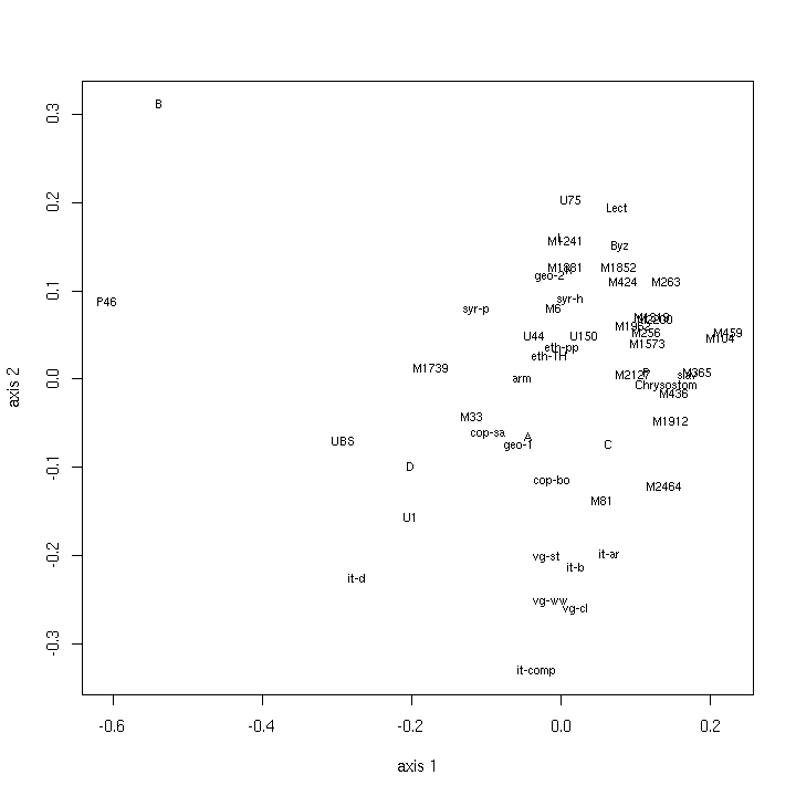
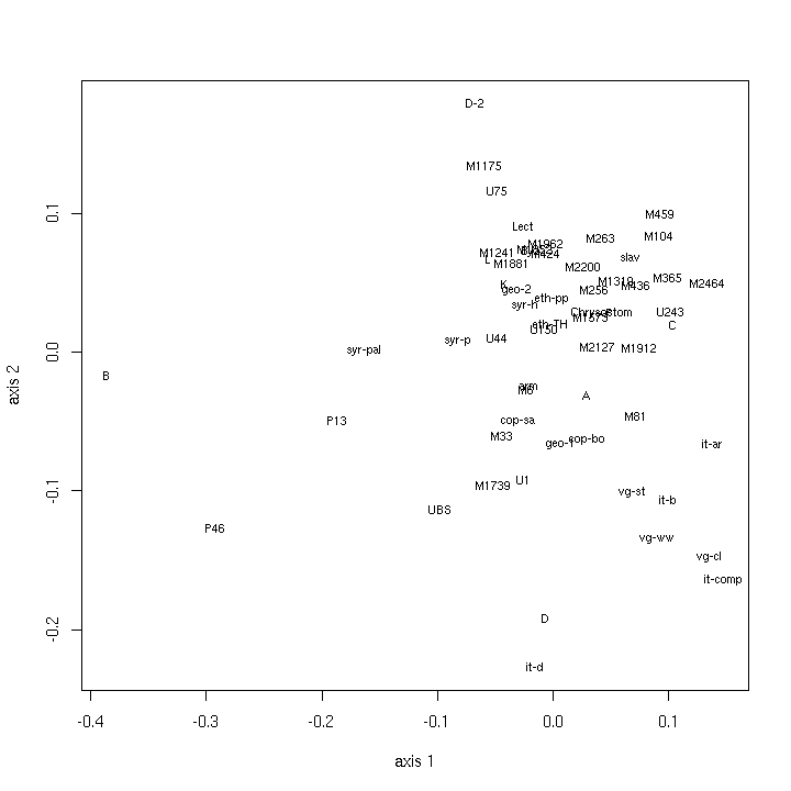
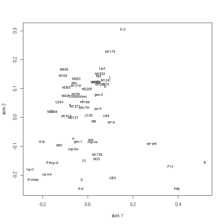
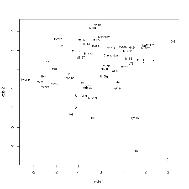
Having been produced by the inclusive strategy, these maps are based on reduced data matrices from which any witnesses that do not share the minimum required number of variation units have been eliminated. As the binary data matrix contains more variation units than the multistate one, the reduced binary data matrix retains more witnesses than the reduced multistate data matrix. Consequently, the three maps based on the binary data matrix contain more witnesses than the map based on the multistate data matrix.
The same set of witnesses is contained in each of the three maps based on the binary data matrix so differences between the maps can be attributed to the respective dissimilarity coefficients. The analysis constructs a dissimilarity matrix from the reduced data matrix before extracting axes which point along directions of maximum variation in the multidimensional space occupied by the witnesses. Small changes in the dissimilarity matrix can affect the directions of the axes and the order in which they are extracted, thereby producing a rotation or reflection when two otherwise similar maps are compared. Consequently, it is sometimes necessary to rotate or reflect one map in order to compare it with another.
The three maps based on the binary data matrix turn out to be quite similar when compared in this way. Taking as a reference the one produced with the simple matching distance, the Jaccard distance map need only have its first axis inverted to show that both maps have similar configurations: witnesses D-2 (i.e. the second corrector of Codex Claromontanus), M1175, and U75 (i.e. majuscule 75) are near the top; B, P46, and P13 are in the lower left quadrant; and the Old Latins and Vulgate are in the lower right quadrant. In a similar fashion, the map based on the Euclidean distance can be made comparable with the simple matching distance map by inverting the first axis then applying a clockwise rotation of about 45 degrees. Whereas the choice of dissimilarity coefficient causes many minor differences, the overall configuration remains the same, apart from rotations and reflections.
The two maps produced with the simple matching distance can be made comparable by rotating the one produced from the multistate data matrix through 45 degrees counterclockwise. Certain witnesses that are present in the map based on the binary data matrix are absent from the one based on the multistate data matrix due to the latter data matrix having fewer variation units. Apart from this difference, these two also have similar configurations.
It is thus apparent that multidimensional scaling produces a similar configuration of points even when the choice of dissimilarity coefficient or type of data matrix is varied. Maps based on a binary data matrix have advantages over their multistate counterparts. For one thing, they are based on more variation units. For another, the Jaccard distance can be used to prevent agreements in absence affecting the result. However, considerable effort is required to convert multistate to binary data. In addition, binary variation units derived from a single multistate variation unit are not independent, making them problematic when it comes to statistical analysis. If results obtained with multistate data are similar to those from binary data then the extra work required to produce a binary representation is hardly justified. In this study, multistate instead of binary data will be used except in cases where the larger number of variation units in the binary data matrix make it preferable to use. The simple matching distance will be used throughout even though there may be advantages to using another distance measure with binary data. This is because a map based on multistate data is more easily compared with one based on binary data if both are produced with the same distance measure.
The last map can be compared with the following one produced with the exclusive strategy, binary data matrix, and Euclidean distance:
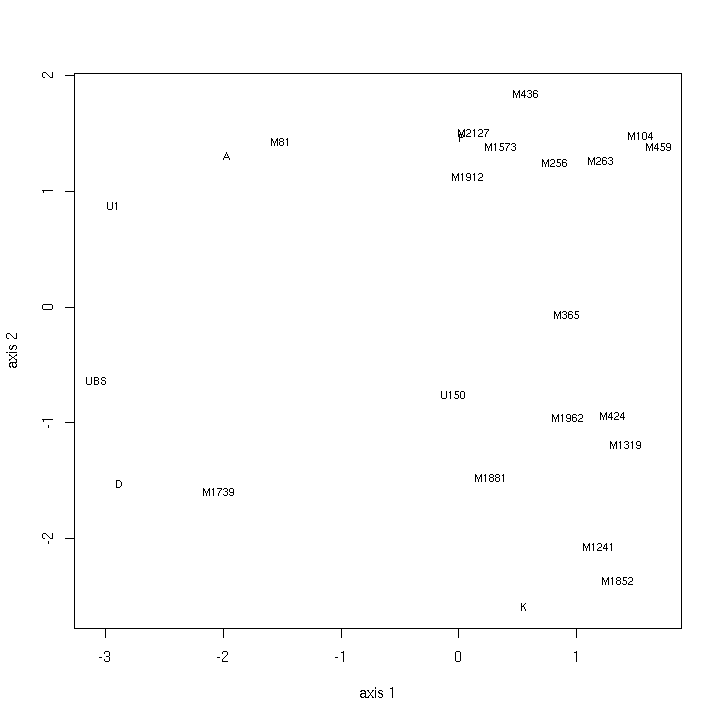
These two differ considerably due to the extra witnesses contained in the map produced with the inclusive strategy. Nevertheless, many similarities remain. Four clusters of witnesses can be seen in the quadrants of the exclusive map:
Upper right: P, M104, M256, M263, M436, M459, M1573, M1912, M2127
Upper left: U1, A, M81
Lower left: D, M1739, UBS
Lower right: K, U150, M365, M424, M1241, M1319, M1852, M1881, M1962
The inclusive map places these clusters of witnesses in close proximity to each other as well.
Comparing the MDS map produced by the exclusive strategy with the “PC2” vs “PC1” plot given in the PCA section, above, shows that the two are identical apart from an inversion of the second axis. An inversion of this kind is inconsequential because the choice of which direction along an axis is regarded as positive is arbitrary. From a mathematical perspective, PCA and MDS are equivalent for binary data if missing data is excluded and Euclidean distance is used for the MDS.
As with PCA, MDS orders map dimensions according to their explanatory power with respect to variation in the input data. The first MDS map dimension thus accounts for more variation than the second, the second for more variation than the third, and so on.
In general, given a set of points in a multidimensional space, the maximum number of dimensions required to plot the points is one less than the number of points. Thus, it takes at most two dimensions to plot three points such as the vertices of a triangle, and three dimensions to accommodate the vertices of a tetrahedron. In some cases, less dimensions are required. For example, three points may lie along a straight line and may therefore be plotted using one instead of two dimensions.
Procedures such as MDS and PCA, which order their axes according to explanatory power, often succeed in accounting for the bulk of variation with fewer than the maximum required number of dimensions. Just how successful they are at achieving this end depends on the inherent dimensionality of the input data. Data that has a low dimensionality can be comprehensively described with fewer dimensions than data with a high dimensionality. The choice of distance measure also affects how adequately a given number of dimensions can account for the total variation of a data set.
The cumulative proportion of variance quantifies the extent to which a given set of axes accounts for variation in the input data. The following table gives cumulative proportions for two dimensions corresponding to the above four MDS maps produced by the inclusive strategy:
| Data | Dissimilarity coefficient | Cumulative proportion |
|---|---|---|
| Multistate | Simple matching | 0.327 |
| Binary | Simple matching | 0.268 |
| Binary | Jaccard | 0.266 |
| Binary | Euclidean | 0.250 |
The multistate simple matching case has the greatest success representing the data, accounting for about one third of the total variation with two dimensions. The binary maps account for about one quarter of the variation, with the simple matching distance doing better than the Jaccard and Euclidean distances. This may be interpreted to mean that the difficulty of representing the underlying data in two dimensions is greatest for the Euclidean distance followed by the Jaccard and simple matching distances.
The dissimilarity between every pair of witnesses contained in an MDS plot is subject to sampling error of the kind discussed in the preceding chapter. It follows that the coordinates of every point plotted in an MDS map are subject to sampling error as well. In general, the larger the number of variation units upon which an MDS map is based, the smaller the relative size of this error.
A confidence region is the multidimensional analogue of the confidence interval for the estimated value of a parameter. In the case of a three-dimensional MDS map, the confidence region associated with a plotted witness location is an ellipsoid. There is more than one way to define such a confidence region ([Cox and Cox] 2001 110-3). As an alternative to the formal analysis required to obtain confidence regions as ellipsoids, this study estimates a margin of error for every plotted point. The result is a spherical confidence region which has a high probability of containing the actual location of the relevant witness. While only an approximation of the confidence region that would be obtained by a formal analysis, it is still a useful indication of the uncertainty associated with a plotted location in an MDS map.
Each witness is located by virtue of its distance from every other mapped witness. The scaling procedure represents a best effort to reproduce these distances in the given number of dimensions. As every distance is uncertain, every plotted location is correspondingly uncertain. We therefore seek a radius for the confidence region surrounding a plotted location which varies according to the uncertainties in all of the distances used to derive the location.
A rough estimate can be obtained by using the quantile function of the binomial distribution to calculate a 95% confidence interval for the proportion of disagreements for every dissimilarity relating to a particular witness. Using a nominal proportion of one half maximizes the width of each interval to produce a conservative result. These interval widths are then divided by the number of variation units for which the witness is defined to obtain a set of relative widths. Taking the square root of the mean of the squares of these values produces a relative interval width specific to the witness in question. Finally, the radius is obtained by multiplying this width by a scaling factor which is the difference between the maximum and minimum values of coordinates in the first dimension.
A three-dimensional representation of a classical MDS map that
incorporates confidence regions of this kind is provided here. It was produced by the script cmds-incl-3d.r
with the multistate data matrix of Hebrews, simple matching distance,
and a minimum of twelve variation units per dissimilarity calculation.
As can be seen from the animated image, the confidence region for a
witness with fewer variation units (e.g. B) is larger than the region
for a witness with more variation units (e.g. P46). This is because the
relative sampling error increases as the number of variation units
decreases.
It is tempting to interpret multidimensional scaling coordinates in terms of more familiar factors. If there is a strong correlation with the place of origin of a witness then a plot of the first two MDS axes should correspond, more or less, to a physical map of Christian population centres around the Mediterranean, and the position of a witness on the map is a hint about the birthplace of its archetype. Time is another potentially important factor. Seeing that the locations and dates of the Church Fathers are often known with some confidence, patristic witnesses make ideal candidates for testing whether correlations exist between multidimensional scaling coordinates and the supposed locations of witnesses and their archetypes in space and time. Manuscripts unearthed from a known location are also valuable in this respect, provided that it is reasonable to assume they were originally copied in or near the same place.
Biplots display both objects and variables on the same plot. There are
a number of types, and the script
biplot.r
uses a popular one named the “principal component
biplot”. This plots objects (i.e. witnesses) according to the
first two principal components but also shows the magnitude and sign of
each variable's contribution to the first two principal components. The
script operates directly on the data matrix so it is necessary to use
binary data. As it employs the exclusive strategy to eliminate missing
data, a reference witness must be specified as well. The following was
produced from the binary data matrix of Hebrews using the UBS text as the
reference witness:
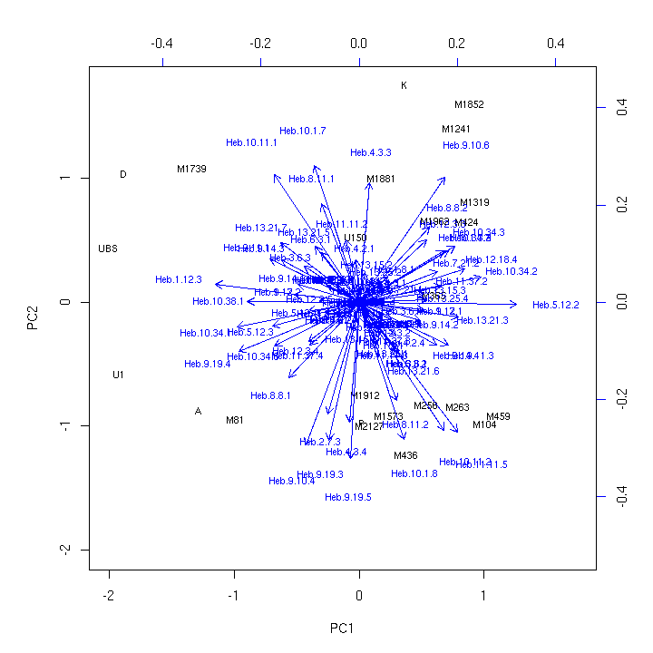
The variables labelled “Heb.5.12.2” and “Heb.1.12.3” are strongly correlated with the first principal component but have opposite signs; variables “Heb.4.3.3” and “Heb.9.19.5” have a similar relationship to the second principal component. Some variables such as “Heb.9.10.8”, “Heb.11.11.5”, “Heb.8.8.1”, and “Heb.10.11.1” make sizable contributions to both the first and second principal components.
Any variables of large magnitude in such a biplot would be suitable for discriminating between witnesses on the basis of the first two principal components. A variable of small or zero magnitude contributes little or nothing to these principal components but may nevertheless contribute to others.
Cluster analysis partitions a set of objects into a number of groups where members of groups are similar to each other but dissimilar to members of other groups. This is not always a straightforward exercise, as indicated by [Chatfield and Collins] (1980 215-6):
An immediate difficulty in cluster analysis is that there is no completely satisfactory way of defining a “cluster”, although we usually have an intuitive idea as to what is meant by the word... [W]e want the clusters to be internally “coherent” but to be isolated from other clusters.
There is another inherent difficulty as well: cluster analysis will always find clusters, regardless of whether any actually exist.
Clustering techniques may be categorized as follows:
agglomerative hierarchical methods, which produce a hierarchy of groups by successively amalgamating smaller groups
divisive methods, which begin with an initial cluster of all objects then produce successive subdivisions
optimal partitioning methods, which partition a set of objects into a predetermined number of groups by optimizing some criterion.
The script named
cluster.r
implements these methods.
Agglomerative clustering begins with individual objects and successively combines them until only one group remains. The result depends on the criterion used to identify the items to combine at each step of the process. Here, an item may be a group of objects or an individual. The following criteria consider the proximity of two groups A and B:
single-link: the minimum distance between an object in group A and one in group B
complete-link: the maximum distance between an object in group A and one in group B
group-average: the average of distances between all possible object pairs, where one object is in group A and the other is in group B.
Other criteria consider something besides proximity. Ward's criterion, for example, combines at each step those two items which produce the least increase of within-group sums of squared distances.
A tree diagram, also known as a dendrogram, displays the hierarchical structure thus generated. The order of dendrogram branches depends on the underlying algorithm. In the present case, the tighter of two clusters is placed on the left.
The following four dendrograms were produced from the multistate data matrix of Hebrews using agglomerative clustering, the inclusive elimination strategy, a minimum of twelve variation units, and the simple matching distance.

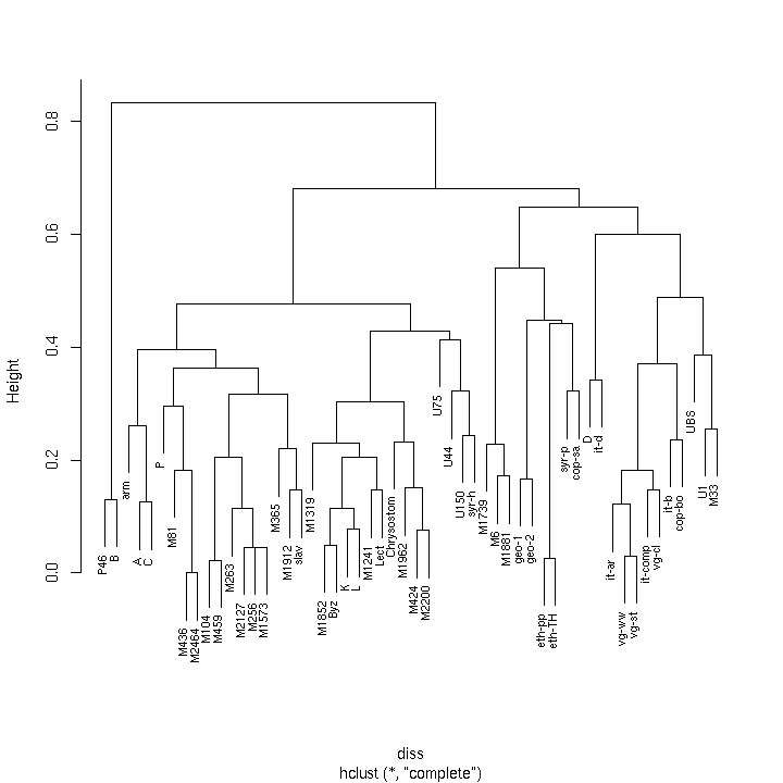
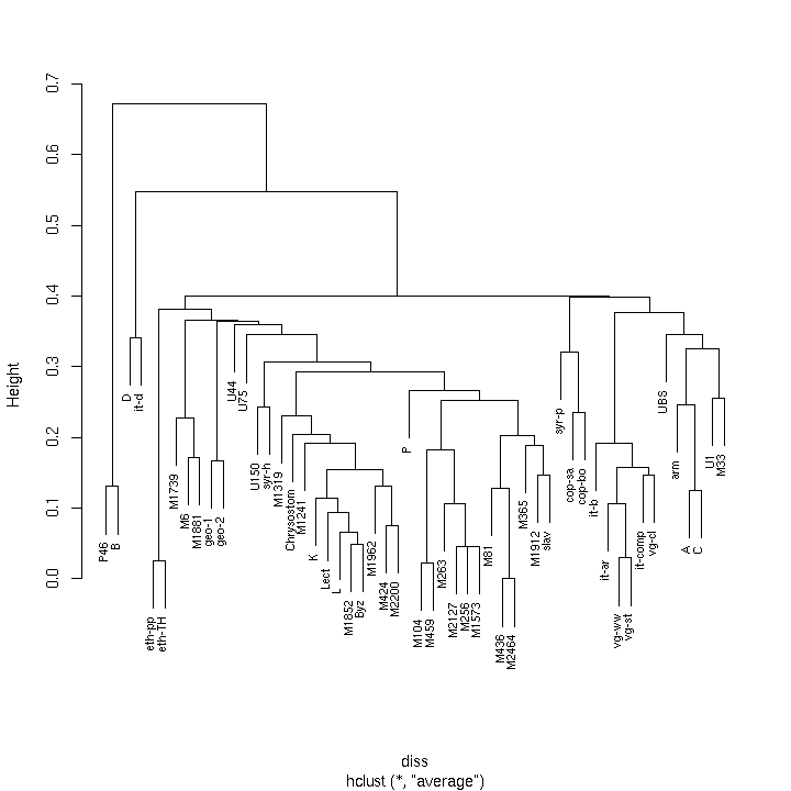
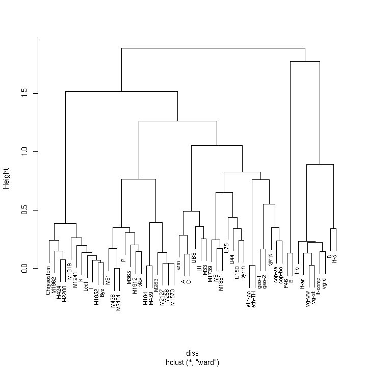
A dendrogram produced by cluster analysis should not be confused with the result of a phylogenetic analysis, which seeks to construct a “family tree” of witnesses. Groups that branch near the top of cluster analysis dendrograms do not have any automatic claims to priority. In this context, isolation is just as well attributed to an eccentric text as to an ancient one.
Dendrograms with a “natural” partition have long-stemmed branches tipped by tight clusters. None of these four dendrograms approach this ideal, although the one produced by Ward's criterion seems to do better than the others. The lack of an obvious partition indicates that there is no preferable number of groups for this data. Should one nevertheless decide to partition the objects, a horizontal line can be drawn across a dendrogram at some point on the vertical axis. To illustrate, the dendrogram produced by Ward's criterion can be “cut” into four groups by a line located at a height of about 1.4 units:
group 1: Chrysostom, M1962, M424, M2200, M1319, M1241, K, Lect, L, M1852, Byz
group 2: M81, M436, M2464, P, M365, M1912, slav, M104, M459, M263, M2127, M256, M1573, arm, A, C, UBS, U1, M33, M1739, M6, M1881, U75, U44, U150, syr-h, eth-pp, eth-TH, geo-1, geo-2, syr-p, cop-sa, cop-bo
group 3: P46, B
group 4: it-b, it-ar, vg-ww, vg-st, it-comp, vg-cl, D, it-d
There is no particular reason for dividing the witnesses into this number of groups. Given the lack of an obvious partition, one might as well choose any number. Four groups are chosen here and in the following examples merely for the purpose of comparing the resultant partitions. Labels assigned to the groups (e.g. “group 1”, “group 2”) are arbitrary.
A divisive clustering method begins with a single group then performs repeated divisions until only individual objects remain. As with the agglomerative method, this approach produces a hierarchical structure that can be displayed as a dendrogram.
The following was produced from the multistate data matrix of Hebrews using the inclusive elimination strategy, at least twelve variation units, and the simple matching distance.
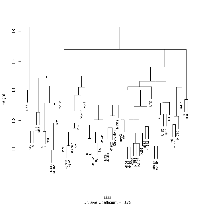
This diagram also indicates that there is no obvious partition for the data set under examination. Indeed, the divisive coefficient, which measures the amount of clustering structure found, is quite small. (A data set with more definite clustering would produce a divisive coefficient closer to one.) The diagram can still be used to partition the data set by cutting the tree at some level. Four groups are produced in the present case by superimposing a horizontal line at a vertical height of about 0.6 units.
group 1: UBS, P46, B
group 2: U1, M33, A, C, M81, M436, M2464, arm, cop-sa, it-ar, vg-ww, vg-st, it-comp, vg-cl, it-b, cop-bo, geo-1
group 3: K, L, M1852, Byz, Lect, M1241, M424, M2200, M1962, Chrysostom, M1319, geo-2, slav, M104, M459, M256, M1573, M2127, M263, M365, M1912, U75, eth-pp, eth-TH, P, U150, syr-h, U44, M6, M1881, M1739, syr-p
group 4: D, it-d
These groups differ from the ones produced by partitioning the Ward's criterion dendrogram into four.
Methods of this class partition the data set into a predetermined number of groups by optimizing some criterion. The method used here searches the data set to find representative objects called “medoids”. Clusters are then constructed by adding objects to their nearest medoids. The optimal partition is the one that minimizes the sum of dissimilarities of group members to their respective medoids.
Setting the desired number of groups to four produces the following result, again using the multistate data matrix of Hebrews, inclusive elimination strategy, at least twelve variation units, and simple matching distance.
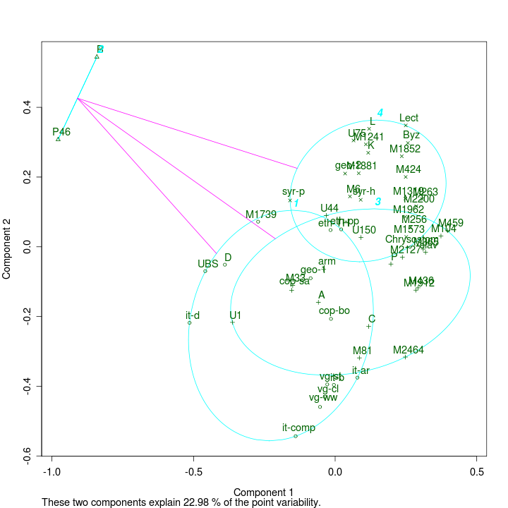
A symbol such as a circle or triangle indicates group membership:
group 1: UBS, D, M1739, it-ar, it-b, it-comp, it-d, vg-cl, vg-ww, vg-st, cop-bo, eth-pp, eth-TH, geo-1
group 2: P46, B
group 3: U1, A, C, P, U44, U150, M33, M81, M104, M365, M436, M459, M1912, M2127, M2464, cop-sa, arm, slav
group 4: K, L, U75, M6, M256, M263, M424, M1241, M1319, M1573, M1852, M1881, M1962, M2200, Byz, Lect, syr-p, syr-h, geo-2, Chrysostom
There are some similarities among the groups produced by the respective clustering techniques but no consensus. The diversity of results implies that this data set does not have an obvious partition. Admittedly, this conclusion only applies to the sample examined here and it is possible that a less ambiguous group structure would emerge if another sample of variation units were analysed.
Classification assigns objects to prespecified classes. A number of multivariate classification methods exist but only one will be demonstrated here. The “k nearest neighbours” technique uses a training data set consisting of a number of objects (i.e. witnesses) that have a known classification. The trained classifier is then used to classify other objects.
The script named
class-knn.r
demonstrates this technique. Firstly, the input data matrix is
reduced using the exclusive strategy because the analysis cannot proceed
if the data matrix contains missing data. Secondly, a dissimilarity matrix
is constructed using Euclidean distance because the k nearest neighbours
technique also uses this dissimilarity coefficient. Next, witnesses in the
reduced data matrix are separated into k groups using medoids extracted by
analysing the dissimilarity matrix. Finally, these k medoids are used to
train the classifier which is then used to classify the witnesses in the
reduced data matrix. The script prints the initial partition and the one
produced by the trained classifier so that the two can be compared.
If the script is configured to classify witnesses into four groups using the binary data matrix of Hebrews and the UBS text as a reference witness then M2127, M436, D, and M1852 are extracted as medoids. These are used to train the classifier which then outputs its classification of the 24 witnesses in the reduced data matrix. In this case, the trained classifier assigns all witnesses except U150 to the same groups as the initial partition. This is a remarkable achievement given that only four witnesses are used to train the classifier.
Whereas classifiers of this kind may seem promising, the quality of a classification depends on the validity of the classes to which the training set are initially assigned. If the data set does not have an obvious partition then there is no obvious set of representative witnesses to train a classifier. A classifier trained with dubious representatives will still make assignments, however meaningless they may be.
A number of groups or “text-types”, such as “Alexandrian”, “Byzantine”, “Caesarean”, and “Western”, have been postulated for New Testament witnesses. In addition, various ad hoc methods have been developed to classify witnesses, some based on levels of agreement with one or more of these text-types; another method forms a “group profile” for an unclassified witness by calculating its levels of agreement with a set of test witnesses.
These methods are almost certainly less effective than multivariate analysis techniques. To give an example, the axis running between “Alexandrian” and “Byzantine” text-types happens to point in roughly the same direction as the first axis obtained by classical multidimensional scaling. Nevertheless, the multidimensional scaling axis has greater classificatory power because it points exactly along the direction of maximum variation. Even so, the above table of proportions of variance informs us that this axis only accounts for about one sixth of all of the variation among the witnesses. A classification scheme based on this axis alone is therefore deficient.
The high dimensionality of the data implies that a group profile method which uses more test witnesses is superior to one which uses less. Indeed, multivariate analysis can identify suitable test witnesses such as the medoids of the optimal partitioning method, but this seems superfluous when multivariate classification techniques can be directly applied to the data.
Another weakness of traditional classification schemes relates to a priori assumptions concerning the number and composition of groups into which New Testament witnesses are thought to fall. It would be better to use a partition derived from the data itself. However, even this is a pointless exercise if the data set does not have a clear group structure, as is indicated by the foregoing analysis of the UBS data for Hebrews. If this result holds when more comprehensive New Testament data sets are analysed then the characterization of witnesses as Alexandrian, Byzantine, Western, or, perhaps, Caesarean will be shown to be arbitrary in the sense that three or four groups is no more preferable than any other possible number.
Table of Contents
- 5.1. Multidimensional scaling maps
- 5.2. General remarks on the maps
- 5.3. The principal map
- 5.4. Other maps
- 5.5. Classification
- 5.6. Witness profiles
- 5.7. Cluster profiles
- 5.8. Temporal correspondence
- 5.9. Geographical correspondence
- 5.10. Results derived from the binary data matrix
- 5.11. Clustering
- 5.12. Are the clusters real?
- 5.13. Textual evolution
- 5.14. Location of the original text
- 5.15. A transmission scenario
- 5.16. Conclusion
Multivariate analysis can be used to survey the space occupied by a set of witnesses. This space has a high dimensionality and its structure can only be fully appreciated by considering all of its dimensions. Fortunately, multivariate analysis often captures much of the information in a few dimensions, making the broad outlines of the distribution of witnesses immediately comprehensible.
The following table provides links to classical MDS maps obtained by analysis of a multistate data matrix derived from the UBS apparatus of Hebrews. Dissimilarities were calculated using the simple matching distance and the inclusive elimination strategy was used to ensure that each calculation was based on at least twelve variation units.
| Reference witness | 2-D map | Prop. of var. (2-D) | 3-D map | Prop. of var. (3-D) |
|---|---|---|---|---|
| Principal | → | 0.327 | → | 0.417 |
| P13 | → | 0.425 | → | 0.525 |
| D-2 | → | 0.371 | → | 0.482 |
| U243 | → | 0.373 | → | 0.489 |
| M1175 | → | 0.375 | → | 0.469 |
| it-v | → | 0.429 | → | 0.566 |
| it-z | → | 0.357 | → | 0.450 |
| syr-pal | → | 0.354 | → | 0.465 |
| cop-fay | → | 0.319 | → | 0.434 |
| Cyril | → | 0.414 | → | 0.530 |
| Theodoret | → | 0.370 | → | 0.465 |
| Ambrose | → | 0.498 | → | 0.647 |
The first row, labelled “Principal”, relates to maps produced when no reference witness is specified. The inclusive elimination strategy starts by dropping all witnesses with less than the required number of variation units, which in the present case has been set at twelve. Next, an iterative cycle begins whereby any witness that does not share enough variation units with some other witness in the remaining set is dropped. As any witness that is dropped during the iterative phase nevertheless has a sufficient number of variation units, it can be specified as a reference witness in order to produce its own maps. This is why the table also includes rows for witnesses P13, D-2, and the rest.
The UBS apparatus does not cover all of the textual variation found among the witnesses. Being based on a limited sample of the entire scope of variation, results obtained by analysing data matrices derived from the apparatus are subject to sampling errors. For this reason, the maps should be regarded as approximations to the actual distribution of witnesses in textual space. Analysis of a more comprehensive set of variation units will produce more precise results. Applying the method to other parts of the New Testament will show whether similar distributions of witnesses occur there.
The maps presented above are two- or three-dimensional projections of a higher-dimensional reality. A feat of mental gymnastics is required when comparing two- and three-dimensional maps for the same reference witness because the first two dimensions form a vertical plane in the two-dimensional maps but a horizontal plane in the three-dimensional ones. In order to see the view presented in a two-dimensional map, an observer must be stationed above the corresponding three-dimensional map.
Given enough dimensions, it is possible to obtain a set of coordinates for each witness such that every distance between witnesses is perfectly represented. However, our faculty for simultaneously comprehending multiple dimensions is limited. While we have no trouble with a two- or three-dimensional representation, perceiving a space with more than three dimensions is more challenging. Devices such as Andrews curves, Chernoff faces, glyphs, and weathervane plots can be employed to convey more information ([Chatfield and Collins] 1980 49-50). Another possibility is to colour plotted points so that red, green, and blue components correspond to coordinate values in the fourth, fifth, and sixth dimensions. However, none of these methods will be pursued here. Instead, the reader should bear in mind that the maps used in this study convey only a part of the full picture.
In general, three-dimensional maps are preferable to their two-dimensional counterparts because they convey more information. The proportion of variance figure shows how much of the underlying proximity information is represented by a map. In the maps provided above, this figure ranges from about one third to one half for two-dimensional maps, and from about four tenths to almost two thirds for the three-dimensional ones. Maps with more dimensions are able to convey more of the total variation than those with less. Also, the proportion of variance explained by a map tends to be higher if it contains fewer witnesses.
Sometimes sigla are superimposed due to proximity of the corresponding witnesses. This problem is aggravated when the analysis is based on a small number of variation units, in which case a number of witnesses can have the same map coordinates. The output of the mapping script includes witness coordinates, allowing superimposed witnesses to be identified. To illustrate, the following table provides coordinates for witnesses in the three-dimensional principal map:
| Witness | Dim. 1 (units) | Dim. 2 (units) | Dim. 3 (units) |
|---|---|---|---|
| UBS | -0.292 | -0.071 | 0.109 |
| P46 | -0.608 | 0.087 | -0.025 |
| U1 | -0.202 | -0.157 | 0.188 |
| A | -0.044 | -0.066 | 0.176 |
| B | -0.538 | 0.311 | 0.121 |
| C | 0.063 | -0.075 | 0.195 |
| D | -0.202 | -0.100 | -0.202 |
| K | 0.011 | 0.123 | -0.113 |
| L | 0.000 | 0.160 | -0.104 |
| P | 0.114 | 0.007 | 0.056 |
| U44 | -0.036 | 0.049 | -0.119 |
| U75 | 0.013 | 0.202 | -0.002 |
| U150 | 0.030 | 0.048 | 0.039 |
| M6 | -0.009 | 0.079 | -0.117 |
| M33 | -0.119 | -0.043 | 0.183 |
| M81 | 0.055 | -0.139 | 0.159 |
| M104 | 0.213 | 0.045 | 0.043 |
| M256 | 0.114 | 0.052 | 0.042 |
| M263 | 0.141 | 0.109 | 0.062 |
| M365 | 0.182 | 0.007 | -0.079 |
| M424 | 0.083 | 0.110 | -0.002 |
| M436 | 0.151 | -0.017 | 0.127 |
| M459 | 0.225 | 0.052 | 0.041 |
| M1241 | 0.006 | 0.156 | -0.031 |
| M1319 | 0.122 | 0.070 | -0.117 |
| M1573 | 0.116 | 0.039 | 0.060 |
| M1739 | -0.174 | 0.012 | -0.058 |
| M1852 | 0.078 | 0.126 | -0.085 |
| M1881 | 0.007 | 0.125 | 0.001 |
| M1912 | 0.147 | -0.048 | 0.025 |
| M1962 | 0.096 | 0.060 | -0.021 |
| M2127 | 0.097 | 0.004 | 0.052 |
| M2200 | 0.126 | 0.067 | -0.084 |
| M2464 | 0.138 | -0.122 | 0.153 |
| Byz | 0.079 | 0.150 | -0.042 |
| Lect | 0.075 | 0.194 | -0.024 |
| it-ar | 0.066 | -0.199 | -0.063 |
| it-b | 0.020 | -0.214 | 0.021 |
| it-comp | -0.031 | -0.332 | -0.024 |
| it-d | -0.272 | -0.226 | -0.286 |
| vg-cl | 0.020 | -0.261 | -0.133 |
| vg-ww | -0.013 | -0.254 | -0.066 |
| vg-st | -0.019 | -0.202 | -0.053 |
| syr-p | -0.113 | 0.077 | 0.019 |
| syr-h | 0.013 | 0.089 | -0.002 |
| cop-sa | -0.098 | -0.064 | 0.188 |
| cop-bo | -0.012 | -0.116 | 0.033 |
| arm | -0.051 | -0.001 | 0.211 |
| eth-pp | 0.003 | 0.034 | -0.087 |
| eth-TH | -0.016 | 0.025 | -0.117 |
| geo-1 | -0.056 | -0.076 | -0.109 |
| geo-2 | -0.014 | 0.116 | -0.007 |
| slav | 0.170 | 0.004 | -0.012 |
| Chrysostom | 0.141 | -0.008 | -0.121 |
Whereas each map is an optimal two- or three-dimensional representation of the given data, it only approximates the higher-dimensional reality. A one-dimensional ordering of witnesses along the first scaling axis is not unlike a conventional characterization of New Testament witnesses that refers to Alexandrian and Byzantine poles. A two-dimensional map encapsulates about twice as much of the associated dissimilarity matrix's proximity information, and three-dimensional maps give another significant improvement in explanatory power. Even so, the three-dimensional maps presented here only convey about one half of the total proximity information. A map may therefore misrepresent the actual distance between two witnesses, and for this reason the relevant dissimilarity matrix should be consulted to determine actual distances between witnesses.
It may be helpful to think of these maps as being like star charts. Two witnesses which seem to be in close proximity may not actually be neighbours, just as two stars which appear to be close to each other may actually be a great distance apart. Their apparent proximity is an illusion which occurs because they lie in approximately the same direction from our point of view. In the same way, even three-dimensional maps can misrepresent the actual distances between witnesses.
Another important consideration is sampling error. Each dissimilarity calculation based on a sample of variation units is subject to this kind of uncertainty. In general, the smaller the number of variation units, the greater the sampling error. As demonstrated in the preceding chapter, an indication of sampling error can be included in a map. Such a plot of the three-dimensional principal map is repeated here. A striking feature of this plot is that most of the confidence regions overlap. From a statistical point of view, it is not safe to say that two witnesses whose confidence regions overlap actually occupy different locations in textual space. Consequently, any identification of specific regions in the following survey of textual space must be regarded as provisional.
An improvement in resolution would be gained by using a larger sample of variation units. The Editio Critica Maior [ECM] being compiled by the Institute for New Testament Textual Research, which includes over three thousand variation units in the Catholic Epistles alone, has great potential in this respect. Returning to the astronomical analogy, the maps might be thought of as badly focused images where each point is diffuse and its exact location ill-defined. As the number of variation units upon which a map is based increases, the focus improves and it becomes easier to resolve witnesses from one another. As the number decreases, the focus gets worse and eventually reaches a point where none of the witnesses can be resolved.
The principal map has a number of regions where witnesses are more concentrated than in other places. These clusters may be no more than random fluctuations in the density of witnesses. In addition, the presence of sampling error makes the location of each witness subject to uncertainty. The following comments on the apparent structure of the textual space occupied by the witnesses of Hebrews included in this survey are therefore tentative and should be treated with due caution. A larger sample of variation units would have to be analysed in order to verify the observations made here.
P46 and B (Vaticanus) are near each other but far removed from the rest. D (Claromontanus) and it-d (the Latin side of Claromontanus) reside in another locality. Witnesses U1 (Sinaiticus), A (Alexandrinus), C (Ephraemi Rescriptus), M33, M81, M2464, arm (Armenian), and cop-sa (Sahidic Coptic) seem to form yet another cluster. Old Latins it-ar, it-b, and it-comp are in a distinct region that includes editions of the Vulgate (vg-cl, vg-st, and vg-ww) as well.
Most of the remaining witnesses are concentrated in a cluster which itself seems to have regions of higher density. However, the magnitude of the sampling error associated with the number of variation units from which the map is constructed makes any assertions about the internal structure of this region highly questionable. Some witnesses, such as M1739, geo-1 (Georgian), cop-bo (Bohairic Coptic), syr-p (Peshitta Syriac), and M436, lie between this cluster and other places of higher density. These witnesses may represent transitional forms, influenced by the texts that lie on either side.
If each witness were considered to be a mass then the centre of mass of all of the witnesses in the map would lie at the origin, where all coordinates are zero. In this map, witnesses U150 and syr-h (Harclean Syriac) are located quite close to the origin. Perhaps unsurprisingly, the UBS text lies almost in the plane defined by P46, U1, and B, but is displaced slightly towards the rest of the witnesses.
The other maps presented above relate to witnesses that have the required minimum number of variation units yet do not appear in the principal map. The map for P13 places it in an isolated location between P46 on one hand and witnesses such as L (Angelicus), U44, and U150 on the other. The second corrector of Claromontanus, D-2, did a thorough job of conforming the text to a Byzantine model similar to K (Mosquensis). U243 lies near witnesses such as M1739 and M1881 while M1175 is near M424. Surprisingly, the Old Latin it-v is nearer to Greek texts such as A (Alexandrinus) and M1881 than to Old Latins it-ar, it-b, it-comp, and it-z. The Palestinian Syriac syr-pal lies near U150 and syr-h. The Fayyumic cop-fay is in the vicinity of the Sahidic (cop-sa) and Bohairic (cop-bo) Coptic texts. The location of quotations by Cyril suggests he used a text similar to the ones preserved in witnesses such as M436, M1912, M2464, and P (Porphyrianus). Theodoret seems to have used a text like that preserved in M1319. The point corresponding to citations by Ambrose is in a remote location beyond witnesses such as it-b and M1739.
Classical scaling coordinates can be used as a basis for classifying witnesses. One approach divides the interval of coordinate values for each dimension into two equal bands thereby producing 2n categories, where n is the number of dimensions. Examining the coordinates of a three-dimensional map would thus produce eight possible categories.
To illustrate this method, the witnesses found in the three-dimensional principal map will be classified according to their scaling coordinates, which are listed above. Once the interval of coordinate values covered by each dimension has been delimited, it is divided into equal bands by reference to a critical value located at the midpoint:
| Dimension | Interval | Band "a" | Band "b" |
|---|---|---|---|
| 1 | -0.608 to 0.225 | x ≤ -0.192 | -0.192 < x |
| 2 | -0.332 to 0.311 | x ≤ -0.011 | -0.011 < x |
| 3 | -0.286 to 0.211 | x ≤ -0.038 | -0.038 < x |
The resulting classifications are shown below:
| Dim. 1 | Dim. 2 | Dim. 3 | Witnesses |
|---|---|---|---|
| a | a | a | D, it-d |
| a | a | b | UBS, U1 |
| a | b | a | None |
| a | b | b | P46, B |
| b | a | a | it-ar, vg-cl, vg-ww, vg-st, geo-1 |
| b | a | b | A, C, M33, M81, M436, M1912, M2462, it-b, it-comp, cop-sa, cop-bo |
| b | b | a | K, L, U44, M6, M365, M1319, M1739, M1852, M2200, Byz, eth-pp, eth-TH, Chrysostom |
| b | b | b | P, U75, U150, M104, M256, M263, M424, M459, M1241, M1573, M1881, M1962, M2127, Lect |
A more precise classification could be obtained by dividing each dimension into more bands. However, any classification scheme of this kind suffers from a significant flaw, which is that witnesses in a region of higher density will be split into separate categories if the region happens to straddle the boundary between adjacent bands.
A better approach would be to classify witnesses according to their location with respect to regions of higher density, as is done by the previously described optimal partitioning technique. The following table shows the result of partitioning the witnesses found in the principal maps into five clusters using this method. There is no particular reason for choosing five clusters instead of another number; if a higher number were chosen then some of the resulting clusters would be similar to these ones but peripheral witnesses would tend to separate.
| Cluster | Medoid | Members |
|---|---|---|
| 1 | vg-ww | UBS, U1, D, it-ar, it-b, it-comp, it-d, vg-cl, vg-ww, vg-st |
| 2 | B | P46, B |
| 3 | M2464 | A, C, P, U44, U150, M33, M81, M104, M365, M436, M459, M1912, M2464, cop-sa, arm, slav |
| 4 | Byz | K, L, U75, M424, M1241, M1319, M1852, M1881, M1962, M2200, Byz, Lect, geo-2, Chrysostom |
| 5 | M2127 | M6, M256, M263, M1573, M1739, M2127, syr-p, syr-h, cop-bo, eth-pp, eth-TH |
A witness with more than twelve variation units which does not appear in the principal maps (i.e. P13, D-2, ..., Ambrose) can also be classified by placing it into the cluster occupied by its nearest already classified neighbour in the relevant entry of chapter four's list of witnesses ordered by dissimilarity. For example, the nearest already classified neighbour of P13 is M424, which is in the fourth cluster. Consequently, P13 is assigned to the fourth cluster as well. The following table adds witnesses assigned by this method in parentheses:
| Cluster | Medoid | Members |
|---|---|---|
| 1 | vg-ww | UBS, U1, D, it-ar, it-b, it-comp, it-d, (it-z), vg-cl, vg-ww, vg-st |
| 2 | B | P46, B |
| 3 | M2464 | A, C, P, U44, U150, M33, M81, M104, M365, M436, M459, M1912, M2464, (it-v), (syr-pal), cop-sa, (cop-fay), arm, slav, (Cyril), (Theodoret) |
| 4 | Byz | (P13), (D-2), K, L, U75, M424, (M1175), M1241, M1319, M1852, M1881, M1962, M2200, Byz, Lect, geo-2, Chrysostom |
| 5 | M2127 | (U243), M6, M256, M263, M1573, M1739, M2127, syr-p, syr-h, cop-bo, eth-pp, eth-TH, (Ambrose) |
Unless history has conspired to deceive us, these clusters correspond to textual families that prevailed in the ancient Christian world; if the clusters are more than random density fluctuations in textual space then they represent actual groupings comprised of like texts whose similarity is presumably due to shared ancestry. Whether this ancestry goes back to a single archetype per cluster would be an interesting topic for future research.
Assuming that these clusters do represent actual groupings, it is natural to seek an explanation for why each one exists. Attributes shared by constituent witnesses can be associated with an entire cluster, providing a means to label clusters in various ways. As an initial step in this process, information concerning date and provenance will be compiled for each witness.
Some classes of witnesses have more potential than others when it comes to identifying the attributes of a cluster. Patristic citations are particularly useful because the dates when and places where a Church Father flourished are often well known. Versions and manuscripts are less useful in this respect but can still provide useful information. The date of a witness is not a direct indication of the dates of the archetypes it preserves. However, the earliest date among the witnesses in a cluster does establish the latest possible date of the archetypal text or texts which gave rise to the cluster.
Similarly, the geographical origin of a constituent witness is not a sure guide to the place where the ancestral text or texts of a cluster arose. As demonstrated by Epp, it was easy for a text produced in one part of the ancient Christian world to be transported to another ([Epp 1991]). In fact, almost every Christian population centre must have received its first texts from other parts of the world. Nevertheless, if dislocation was the exception rather than the rule then it is worth taking note if there is a prevailing vote among constituent witnesses whose birthplaces can be established.
Information concerning the date and provenance of a witness is often imprecise and speculative, if it exists at all. Nearly all biblical manuscripts are dated by palaeographical considerations. The margin of error associated with such a dating, though rarely stated, is often not better than plus or minus half a century. Place of recovery, scribal characteristics, annotations, and textual similarity to patristic citations provide clues about the provenance of a witness but none of these is a sure guide.
The following table brings together opinions on dates and provenances of a number of witnesses included in the maps. Apart from the Old Latin version and M1739, dates are as given in the fourth edition of the [UBS] Greek New Testament, with cardinal numerals referring to centuries. For M1739, the date and provenance relate to the exemplar from which it is thought to have been copied. Unless otherwise indicated, the provenance of a versional witness is taken to be the main locality where its language was spoken.
| Witness | Date (A.D.) | Provenance | Comments |
|---|---|---|---|
| P13 | 3rd/4th | Egypt | Recovered from Egypt. |
| P46 | about 200 | Egypt | Recovered from Egypt. |
| Sinaiticus (U1) | 4th | Egypt ([Ropes] 1926 xlvii-xlviii); Palestine ([Milne and Skeat] 1938 69) | |
| Alexandrinus (A) | 5th | Egypt ([Ropes] 1926 li-liii); Constantinople (Burkitt); Caesarea or Berytus ([Streeter] 1930 120) | Burkitt's opinion is mentioned by Streeter in the work cited. |
| Vaticanus (B) | 4th | Egypt ([Ropes] 1926 xxxiv-xxxvi) | |
| Ephraemi Rescriptus (C) | 5th | Egypt ([Milne and Skeat] 1938 67); Constantinople (Tischendorf) | According to [Lyon] (1958 19), “Critics have generally voiced their hesitancy to locate Codex C.” While [Ropes] (1926 lv) reports that Tischendorf thought the manuscript may have been in Constantinople when it was repurposed, he says that “There seems to be no sufficient reason for any confident assertion that it is of Egyptian origin.” MDS maps of substantive and orthographic variations are consistent with this codex having a Byzantine spelling of an Egyptian text ([Finney 1999]). |
| Claromontanus (D 06) | 6th | Sardinia ([Souter] 1954 26) | This Greek-Latin diglot codex is written in sense lines. According to [Souter] (1954, 26), “with the exception of harmonizations with the Vulgate Latin text in the longer Epistles, the Latin side is precisely the same text as Lucifer of Cagliari (in Sardinia) uses in his writings in the fourth century”. |
| M1739 | 4th (presumed date of exemplar) | Caesarea (presumed provenance of exemplar) | [Zuntz] (71-73) writes that this manuscript was copied by the monk Ephraim about the middle of the tenth century. The Pauline Epistles preserve the text of an ancient exemplar along with marginal notes identifying agreements and disagreements with the text of Origen. Zuntz says that the ancient exemplar stands in the best Eusebian tradition of philology, and believes it was produced in Caesarea “hardly later than c. A.D. 400.” |
| Old Latin (it-ar, it-b, it-comp, ...) | 3rd | Europe |
While late second century Latin translations of parts of the New Testament existed, the first evidence of an identifiable Latin text-type is found in mid-third century quotations by Cyprian of Carthage. This “African” version, which may in fact have come from Italy, was revised to produce a “European” tradition, evidence of which is found in a number of fourth century writers. ([Petzer] 1995 120-1) |
| Vulgate (vg-cl = Clementine; vg-ww = Wordsworth-White; vg-st = Stuttgart) | 4th, 5th | Palestine | Based on the Old Latin and compared with Greek manuscripts, Jerome finished his revision of the Gospels around 383 A.D. No one knows who revised the rest of the New Testament or when. ([Metzger 1992] 76; [Petzer] 1995 123) |
| Coptic (cop-sa = Sahidic; cop-bo = Bohairic; cop-fay = Fayyumic) | 3rd | Egypt | The Sahidic dialect of Coptic was in literary use throughout Egypt while the Bohairic was associated with the Nile delta and the Fayyumic with the Fayyum Oasis. ([Metzger 1977] 106) |
| Ethiopic (eth-pp = Pell Platt; eth-TH = Takla Haymanot) | about 500 | Ethiopia | Translated from fourth or fifth century Greek manuscripts. ([Zuurmond] 1995 153) |
| Syriac (syr-p = Peshitta; syr-h = Harclean) | first half of 5th (syr-p); 616 (syr-h) | Syria (syr-p); Egypt (syr-h) | The Peshitta was the eventual result of a revision of the Old Syriac instituted by Rabbula, bishop of Edessa, early in the fifth century. The Harclean was produced by Thomas of Harkel in 616 A.D. at Enaton near Alexandria. ([Aland and Aland] 1989 194-9; [Metzger 1992] 69-71) |
| Palestinian Aramaic (syr-pal) | about the sixth century | Palestine | It is hard to say when or where the Palestinian Syriac came from. An Aramaic text written with a Syriac script, its language suggests a Palestinian, Syrian, or even Egyptian place of origin. ([Aland and Aland] 1989 199) |
| Armenian (arm) | 5th | Armenia | The Armenian version was produced in the fifth century through the efforts of Mesrop, Sahak, and others. An initial translation was made from an Old Syriac base text early in the fifth century. This was thoroughly revised using Greek manuscripts brought from Constantinople after the Council of Ephesus, held in 431 A.D. ([Alexanian] 1995 157) |
| Georgian (geo-1, geo-2) | 5th (geo-1) | Georgia | A first translation into Georgian (geo-1), which may have been based on the initial Armenian translation, was superseded by a revision against Greek manuscripts (geo-2). The latter was made some time after the Georgian and Armenian churches separated in the early seventh century. ([Aland and Aland] 1989 205) |
| Old Church Slavonic (slav) | 9th | Europe | Produced by brothers Constantine (that is, Cyril) and Methodius of Thessalonika using a Greek model. ([Metzger 1992] 85) |
Details of where the other witnesses included in the maps might have been produced are difficult to find in reference books. The manuscripts themselves sometimes contain relevant clues in the form of scribal annotations and colophons. Along with the usual palaeographical and codicological details, it would be helpful for manuscript catalogues to include such indications as well.
The five way partition of witnesses and preceding witness profiles are brought together in the following table. In most cases, the date given for a cluster is that of the earliest among its constituent witnesses; in the case of the first cluster, it is the presumed date of the earliest representatives of the Old Latin version. If opinions on the date or provenance of a witness vary then it may appear in support of more than one cluster date or region, as does Sinaiticus (U1) for the first cluster region.
| Cluster | Members | Latest date (A.D.) | Regions | |
|---|---|---|---|---|
| 1 | UBS, U1, D, it-ar, it-b, it-comp, it-d, (it-z), vg-cl, vg-ww, vg-st | late 2nd (Old Latins) | Europe (Old Latins); Egypt (U1); Palestine (U1) | |
| 2 | P46, B | about 200 (P46) | Egypt | |
| 3 | A, C, P, U44, U150, M33, M81, M104, M365, M436, M459, M1912, M2464, (it-v), (syr-pal), cop-sa, (cop-fay), arm, slav, (Cyril), (Theodoret) | 3rd (Coptic) | Egypt (A, C, cop-sa, cop-fay, Cyril); Palestine (A, syr-pal); Syria (A, Theodoret); Constantinople (C); Europe (it-v, slav); elsewhere (arm) | |
| 4 | (P13), (D-2), K, L, U75, M424, (M1175), M1241, M1319, M1852, M1881, M1962, M2200, Byz, Lect, geo-2, Chrysostom | 3rd/4th (P13); late 4th (Chrysostom) | Egypt (P13); Syria (Chrysostom); Constantinople (Chrysostom) | |
| 5 | (U243), M6, M256, M263, M1573, M1739, M2127, syr-p, syr-h, cop-bo, eth-pp, eth-TH, (Ambrose) | 3rd (cop-bo); late 4th (Ambrose); early 5th (syr-p) | Egypt (cop-bo, syr-h); Syria (syr-p); Europe (Ambrose); elsewhere (Ethiopic) |
Going by the dates of a cluster's earliest witnesses, the first and second clusters would seem to be more ancient than the others. However, as the old maxim says, a late witness may preserve an early text, and vice versa. If clusters represent the descendants of a few archetypal texts then the only significant dates are those of the archetypes. As far as cluster profiles are concerned, what matters is the earliest date among constituent witnesses, which represents the latest possible date for the grouping preserved by the cluster. The actual dates of these clusters' archetypal texts may be significantly earlier than the earliest dates among their surviving witnesses.
Rather than focus on the correspondence between clusters and dates, it might be more fruitful to investigate the evolution of clusters with time. One can imagine animating a scaling map so that each witness siglum was highlighted during frames corresponding to its probable date range. If the animation showed a general diffusion away from some location then it would be reasonable to associate that location with earlier forms of the text.
Once again, it needs to be stated that sampling errors make any assertions based on these analysis results provisional and that larger samples should be examined to verify the observations made here. That said, there appears to be a broad correspondence between cluster membership and geographical provenance. In fact, three-dimensional scaling maps can often be rotated so that cluster locations in a two-dimensional projection correspond to the physical locations of early Christian centres of literary activity. For example, if the particular orientation of the three-dimensional principal map shown here were superimposed on a physical map of the Mediterranean, the majority of witnesses in the third cluster would lie in locations corresponding to Egypt and Palestine, most witnesses in the fourth cluster would have locations corresponding to Syria, those of the fifth cluster would mainly occupy locations associated with Palestine or Syria, while most witnesses in the first cluster would be to the “west” of the other clusters.
This rather astonishing result was long ago anticipated by Streeter with his theory of local texts. Citing graduated levels of agreement between witnesses, he gave an interpretation of the evidence which associates groupings with localities ([Streeter] 1930 106):
If we look at the [physical] map we see at once that the Churches whose early texts we have attempted to identify stand in a circle round the Eastern Mediterranean--Alexandria, Caesarea, Antioch, (Ephesus), Italy-Gaul, and Carthage. The remarkable thing is that the texts we have examined form, as it were, a graded series. Each member of the series has many readings peculiar to itself, but each is related to its next-door neighbour far more closely than to remoter members of the series...
Antecedently, we should rather expect the text of any particular locality to be, up to a point, intermediate between those of the localities geographically contiguous with it on either side. But the exactness of correspondence between the geographical propinquity and the resemblance of text exceeds anything we should have anticipated.
Perhaps if multivariate analysis had been available in his time, Streeter would have used scaling maps as evidence in support of his theory.
Admittedly, some witnesses occupy locations that go against a geographical reading of the evidence. Given the physical location of Armenia, the Armenian version might be expected to lie somewhere besides a cluster associated with Egypt or Palestine. However, its seemingly incongruous location can be understood once it is recalled that the Armenian version was revised against Greek manuscripts brought from Constantinople about 431 A.D. If these manuscripts had the same kind of text as preserved in witnesses of the third cluster then the Armenian version would not be out of place.
[Streeter] (1930 102-5) suggested that the fifty Bibles ordered by Emperor Constantine from Eusebius of Caesarea around 331 A.D. were eventually displaced by copies of the standard Byzantine text later preferred in Constantinople. Desiring clean copies, richer churches would give or sell their deluxe yet deprecated volumes to provincial churches and monasteries. In this way, so Streeter speculated, one of the fifty may have come into the hands of Mesrop and Sahak who then used it to revise their translation. If the revised Armenian indeed reflects the text of the fifty Bibles commissioned by Constantinople then the third cluster preserves a text that would have been familiar to Eusebius.
Strict geographical correspondence would require the Ethiopic version, here represented by the Pell Platt (eth-pp) and Takla Haymanot (eth-TH) editions, to be located far from its actual location in textual space. Some hold that the Ethiopic version was influenced by Syrian Monophysites who fled to Egypt after being condemned at the Council of Chalcedon in 451 A.D. [Zuurmond] (1995 148) agrees that there is a Syrian influence, but regards it as having occurred at a much later time. Whenever the date of the influence, the Ethiopic version's textual location does suggest that it conforms to a text associated with Syria.
Historical circumstances could also account for the locations of a number of other witnesses whose supposed places of origin do not coincide with their positions in textual space. Two representatives of the Georgian version are included in the maps, with the text preserved in the first (geo-1) thought to predate that of the second (geo-2), which was supposedly revised against Greek manuscripts. Referring to the specific map orientation mentioned above, geo-1 might then be expected to lie to the “east” (i.e. right) of Chrysostom. If not an artifact caused by sampling error, the actual location of this text may be due to the source from which it was translated, possibly the initial Armenian version. If the initial Armenian was in turn translated from the Old Syriac then the position of geo-1 is a clue to where the initial Armenian and Old Syriac were located in textual space. The other representative of the Georgian version (geo-2) included in these maps lies in a place that indicates it was edited to conform to the standard Byzantine text preserved in Greek witnesses such as K and M424. The location of the Old Church Slavonic (slav) indicates that it was translated from a text of the kind preserved in M1912.
The text of the Vulgate is represented here by the Clementine (vg-cl), Wordsworth-White (vg-ww), and Stuttgart (vg-st) editions. No one knows who edited the version of Hebrews found in the Vulgate. If it was Jerome, or someone else working with him in Palestine, then its text might be expected to lie in a cluster associated with Palestine rather than one associated with Europe. However, we should instead expect the Vulgate to occupy a position in textual space near Old Latin texts of the kind from which it was produced, as it does. In general, the textual location of a witness is determined by its sources. If there is a correspondence between textual location and geographical provenance then it applies to the archetypal texts from which the cluster arose and does not necessarily apply to all of the constituent witnesses.
The second cluster (P46, B) also seems to admit a geographical reading of the data, although not with the particular orientation of the three-dimensional principal map already used. This illustrates a basic weakness of a geographical interpretation, which is its inherent limitation to only two dimensions. While a three-dimensional treatment is better, it still falls short of accounting for all of the underlying dissimilarity information.
This study constrains the minimum number of variation units required for a dissimilarity calculation in order to reduce sampling errors to a tolerable level. While necessary, the constraint causes many witnesses to be excluded from analysis results. As a class, the Church Fathers are particularly badly affected in this respect, with only a few represented in scaling maps derived from the multistate data matrix. This is unfortunate because patristic citations are valuable when it comes to associating parts of textual space with known dates and locations. Happily, by using the binary data matrix instead of the multistate one, it is possible to extract data for a number of additional witnesses. The following table presents lists of witnesses ordered by dissimilarity based on the binary data matrix, inclusive elimination strategy, simple matching distance, and a constraint of at least twelve variation units per dissimilarity calculation. While having the advantage of not counting agreements in absence, the Jaccard distance is not used to avoid reducing the number of variation units from which a dissimilarity is calculated below the required minimum.
| Reference witness | Nearest to farthest witnesses |
|---|---|
| U1-2 | M1739, M1852, Chrysostom, M104, M459, M1881, M424, M1319, M1962, M2200, vg-st, syr-h, cop-bo, P46, U44, M81, it-ar, it-b, it-comp, L, P, M1241, M1912, Byz, Lect, D-2, U150, M256, M263, M436, M1573, M2127, vg-ww, cop-sa, slav, M33, A, K, M365, geo-1, M2464, UBS, vg-cl, arm, geo-2, U75, eth-pp, eth-TH, U1, D, it-d |
| H | vg-cl, vg-ww, vg-st, UBS, geo-1, A, arm, U150, M33, M81, M1739, U44, M1962, it-ar, M1912, M2127, it-b, it-comp, Chrysostom, M6, U1, M436, P, M1573, it-z, syr-h, D, K, M424, M1852, it-d, Byz, P46, M104, M256, M365, L, syr-p, geo-2, M263, M459, M1319, M1881, Lect, slav, M1241 |
| I | M33, M256, M1573, M2127, cop-sa, cop-bo, UBS, U1, P, M81, M263, M436, M1881, M1912, it-b, arm, A, K, M2464, it-comp, M104, M459, L, M365, M424, vg-cl, vg-ww, vg-st, M2200, Byz, Lect, geo-2, slav, Chrysostom, it-ar, D-2, U150, M1241, M1319, M1739, M1852, M1962, syr-h, geo-1, eth-pp, eth-TH, P46, B, U75, it-d, D |
| U48 | M33, M81, U1, it-b, it-comp, it-z, cop-bo, P13, P46, L, P, M1739, A, U150, it-ar, UBS, D, K, M6, M104, M256, M263, M365, M424, M436, M459, M1319, M1573, M1852, M1881, M1912, M1962, M2127, M2200, Byz, Lect, syr-p, cop-sa, arm, geo-1, geo-2, slav, Chrysostom, D-2, M1241, it-d, U44, eth-pp, eth-TH |
| U75-supp | geo-2, M1241, M1319, Lect, Byz, slav, M104, M256, M1881, U1, K, L, M263, M459, M1852, it-z, D, P, M33, M81, M1573, it-ar, it-b, it-comp, Chrysostom, syr-h, geo-1, M424, M436, it-d, it-r, UBS, A, M1739, M1912, M2127, vg-cl, vg-ww, vg-st, arm, syr-p, H, P46, M1962, U150, M365 |
| M424-c | M6, M1739, it-b, it-comp, M1881, eth-pp, eth-TH, M1573, M2127, syr-h, it-ar, vg-cl, vg-ww, vg-st, P46, D, U150, Chrysostom, UBS, M256, cop-sa, cop-bo, geo-1, it-d, M263, B, D-2, U44, M2200, syr-p, L, A, M33, M81, M1912, arm, U75, Byz, K, M1241, M104, M365, M1962, geo-2, Lect, U1, P, M459, M1852, slav, M2464, M424, M436, M1319, M1175 |
| L593 | P, M365, M1912, it-comp, eth-TH, M104, M436, M459, M1962, vg-cl, M2200, slav, A, M81, it-ar, it-d, vg-ww, vg-st, syr-p, cop-sa, eth-pp, D, M424, M1319, Chrysostom, UBS, it-b, cop-bo, K, U150, M256, M263, M1573, M1739, M1852, M2127, arm, P46, U1, M33, syr-h, geo-1, L, M1241, Byz, Lect, M1881, geo-2 |
| L596 | M104, M436, M459, M2464, P, M1912, M365, M81, M256, M263, M1573, M2127, eth-pp, eth-TH, cop-sa, cop-bo, arm, it-comp, slav, M1962, M2200, U75, it-b, U1, A, M1739, M1881, UBS, P46, D, M424, M1319, Chrysostom, it-ar, M33, geo-1, B, it-d, M1852, syr-h, geo-2, K, L, U150, M1241, Byz, Lect |
| L1441 | M1912, P, A, M436, M2464, M104, M424, M459, M1962, M2200, eth-TH, UBS, M81, M365, arm, geo-1, M256, M263, M1319, M1573, M2127, syr-p, eth-pp, U1, D, it-d, geo-2, K, U150, M33, M1739, M1852, Byz, Lect, syr-h, Chrysostom, L, M1241, M1881 |
| it-mu | M81, it-b, UBS, M6, M33, M1912, M2127, it-comp, arm, A, D, U150, M1739, it-ar, P46, U44, M436, M1573, it-d, Chrysostom, M365, M424, M1962, it-r, U1, P, M104, M256, K, L, M263, M459, M1175, M1241, M1319, M1852, Byz, Lect, slav, M1881 |
| it-r | UBS, it-d, it-z, vg-cl, vg-ww, vg-st, U44, P46, M1739, H, U1, M33, it-comp, geo-1, K, L, M81, M1852, M1962, Byz, it-ar, M436, M1881, arm, Chrysostom, geo-2, A, U150, M424, M1241, M1319, Lect, it-b, U75-supp, slav, P, M104, M256, M365, M1912, M2127, D, M263, M459, M1573, syr-h, syr-p |
| it-t | it-ar, it-b, it-comp, M81, M365, M436, M2464, U150, M33, M1962, it-d, arm, geo-1, cop-bo, slav, U1, A, L, P, M104, M256, M263, M424, M459, M1241, M1852, M2127, M2200, Byz, Lect, Chrysostom, cop-fay, D, M1573, M1881, M1912, geo-2, UBS, K, U75, M1319, syr-h, eth-pp, eth-TH, syr-p, M1739, P46 |
| it-v | C, A, vg-st, M81, M436, M2464, P, U44, U75, U150, M33, M256, M263, M365, M2127, it-ar, arm, vg-ww, syr-pal, M1573, M1881, M104, M459, M1912, M1962, it-b, syr-h, slav, cop-bo, Lect, K, L, M424, M1241, M1852, M2200, Byz, vg-cl, UBS, it-comp, syr-p, eth-pp, eth-TH, geo-1, Chrysostom, U1, U243, M6, geo-2, B, M1739, M1319, cop-sa, D, it-d, P46 |
| it-z | it-b, it-comp, it-ar, cop-bo, vg-ww, vg-st, it-d, M81, M1739, Byz, M1319, Lect, M256, M424, M2127, M6, D-2, slav, M33, geo-2, U1, M263, M436, M1912, Chrysostom, M2200, vg-cl, UBS, A, P, M104, M1573, M1852, M1962, P46, M459, M1881, geo-1, U44, K, U150, M1241, eth-pp, eth-TH, arm, L, syr-h, M1175, M365, cop-sa, syr-p, D |
| cop-fay | cop-sa, cop-bo, M256, M2127, M263, M1573, M1912, A, P, M33, M104, M424, M459, arm, it-comp, M436, it-b, M2464, syr-p, it-ar, eth-pp, eth-TH, M81, slav, Lect, U1, M1881, M2200, syr-h, geo-2, UBS, M1962, Byz, geo-1, K, M1241, M1319, vg-cl, vg-ww, vg-st, U150, M1739, it-d, Chrysostom, B, L, M365, M1852, U44, U75, P46, D |
| Clement | M365, M424, M436, M1962, geo-2, D-2, U1, K, L, M263, M459, M1319, M1852, Byz, Lect, it-comp, arm, slav, eth-pp, eth-TH, it-ar, P, U44, M104, M256, M1241, M1912, M2127, A, U150, M6, M33, M1881, cop-sa, cop-bo, geo-1, it-z, UBS, P46, M81, M1573, M1739, it-b, it-d, Chrysostom, syr-h, D |
| Cyril | M436, M1912, slav, vg-st, P, U150, M81, M1962, M2200, M2464, Chrysostom, U44, vg-cl, vg-ww, arm, M104, M424, M459, M1319, M1852, cop-sa, M33, M365, K, M256, M1241, M2127, Byz, it-ar, L, UBS, M263, M1573, Lect, geo-1, cop-bo, eth-pp, eth-TH, syr-h, it-b, it-comp, A, geo-2, C, U75, M1881, syr-p, U1, it-d, M6, D, U243, B, M1739, P46 |
| Didymus | A, M104, M256, M263, M436, M459, M1573, M1881, M1912, M2127, arm, cop-bo, UBS, cop-sa, P, M33, M81, M1241, syr-p, K, M424, M1852, Byz, Lect, it-comp, geo-2, Chrysostom, slav, M2200, U1, U150, M1739, it-b, it-d, U44, M6, vg-cl, vg-ww, vg-st, L, M1319, M1962, syr-h, geo-1, eth-pp, eth-TH, it-ar, M365, P46, U75, D, Ambrose |
| Eusebius | M1241, eth-pp, eth-TH, A, K, M104, M256, M263, M365, M424, M459, M1319, M1573, M1852, M1881, M1912, M1962, M2127, Byz, Lect, cop-sa, slav, Chrysostom, M436, it-comp, arm, UBS, P46, L, P, U150, M1739, it-d, geo-1, geo-2, M33, M81, it-b, U1, syr-h, D |
| Gregory-Nyssa | P, U150, M256, M263, M1319, M2127, M2200, it-ar, it-b, it-comp, vg-cl, vg-ww, vg-st, Chrysostom, M1573, A, K, M33, M81, M104, M424, M436, M459, M1241, M1852, M1881, M1912, M1962, it-d, syr-h, arm, slav, UBS, U1, D, M1739, geo-1, geo-2, M365, syr-p, P46 |
| John-Damascus | M1881, Lect, L, M104, M424, M459, M1241, M1852, M1962, Byz, Chrysostom, M2200, M263, U1, A, K, P, U150, M33, M81, M256, M436, M1573, M1912, M2127, arm, slav, syr-h, Cyril, M1739, geo-2, UBS, M1319, it-comp, vg-cl, vg-ww, vg-st, syr-p, it-ar, M365, geo-1, it-b, it-d, P46, D |
| Origen | M104, M256, M263, M424, M436, M459, M1319, M1573, M1852, M1912, M1962, M2127, M2200, Byz, Lect, it-ar, it-b, it-comp, arm, slav, Chrysostom, vg-cl, vg-ww, vg-st, Cyril, U150, M1241, M1881, it-d, L, A, K, U1, P, M365, M1739, M33, M81, geo-1, geo-2, UBS, D, P46 |
| Theodoret | P, M1175, M256, M263, M365, M2127, syr-h, A, M1573, M1912, U44, M2200, K, U150, it-comp, syr-p, UBS, M33, M436, M1319, arm, eth-TH, M6, cop-sa, slav, M81, M104, M424, M459, M1739, geo-2, D-2, cop-bo, vg-cl, vg-ww, vg-st, Lect, Byz, M1241, M1962, it-ar, it-b, eth-pp, Chrysostom, L, D, M1852, it-d, M1881, geo-1, U1, P46 |
| Ambrose | P46, B, M1739, it-d, eth-pp, eth-TH, M6, syr-pal, cop-sa, cop-bo, UBS, K, M256, M1573, M1881, M2127, it-b, Byz, Lect, geo-1, geo-2, U150, M1241, it-comp, L, M263, M424, arm, it-ar, Chrysostom, vg-cl, vg-ww, vg-st, A, M33, syr-h, M104, M365, M436, M459, M1319, M1852, M1912, M1962, M2200, syr-p, slav, U1, U44, P, M81, U75, C, D, M2464 |
| Augustine | K, L, M424, M1852, M2200, Byz, Lect, slav, M256, M263, M365, M1241, M1319, M1573, M1912, M2127, Chrysostom, it-comp, vg-ww, vg-st, geo-2, A, M6, M33, M104, M436, M459, M1739, M1881, M1962, arm, eth-pp, eth-TH, UBS, D, geo-1, it-b, it-d, vg-cl, U44, U75, U1, P, M81, P46, U150 |
| Jerome | L, syr-h, U150, K, P, M33, M81, M104, M256, M263, M365, M424, M436, M459, M1852, M1912, M1962, M2127, Byz, Lect, cop-bo, arm, geo-2, slav, Chrysostom, M2200, M1241, M1573, M1881, cop-sa, U75, U1, A, U44, M1319, it-comp, it-d, geo-1, it-ar, UBS, M6, eth-pp, eth-TH, it-b, M1739, D, P46 |
| Lucifer | it-b, it-comp, vg-cl, it-ar, vg-ww, vg-st, P46, U1, A, C, U243, M1739, it-d, it-v, geo-1, UBS, P13, B, D, U75, M6, M81, M104, M256, M263, M365, M436, M459, M1573, M1881, M2127, syr-p, eth-pp, eth-TH, geo-2, M2464, K, L, P, U44, U150, M33, M424, M1241, M1319, M1852, M1912, M1962, M2200, Byz, Lect, syr-h, syr-pal, arm, slav, Chrysostom |
Corresponding classical MDS maps are presented in the following table:
| Reference witness | 2-D map | Prop. of var. (2-D) | 3-D map | Prop. of var. (3-D) |
|---|---|---|---|---|
| Principal | → | 0.268 | → | 0.351 |
| U1-2 | → | 0.403 | → | 0.502 |
| H | → | 0.461 | → | 0.589 |
| I | → | 0.361 | → | 0.493 |
| U48 | → | 0.479 | → | 0.601 |
| U75-supp | → | 0.531 | → | 0.664 |
| M424-c | → | 0.323 | → | 0.425 |
| L593 | → | 0.388 | → | 0.520 |
| L596 | → | 0.423 | → | 0.556 |
| L1441 | → | 0.530 | → | 0.670 |
| it-mu | → | 0.742 | → | 0.808 |
| it-r | → | 0.455 | → | 0.577 |
| it-t | → | 0.419 | → | 0.549 |
| it-v | → | 0.378 | → | 0.511 |
| it-z | → | 0.310 | → | 0.405 |
| cop-fay | → | 0.328 | → | 0.439 |
| Clement | → | 0.458 | → | 0.592 |
| Cyril | → | 0.363 | → | 0.466 |
| Didymus | → | 0.405 | → | 0.546 |
| Eusebius | → | 0.609 | → | 0.741 |
| Gregory-Nyssa | → | 0.781 | → | 0.915 |
| John-Damascus | → | 0.552 | → | 0.717 |
| Origen | → | 0.533 | → | 0.676 |
| Theodoret | → | 0.363 | → | 0.453 |
| Ambrose | → | 0.417 | → | 0.510 |
| Augustine | → | 0.419 | → | 0.547 |
| Jerome | → | 0.558 | → | 0.676 |
| Lucifer | → | 0.573 | → | 0.686 |
The witnesses will again be partitioned into five clusters. As before, any mapped witness that does not appear in the principal maps is assigned to the same cluster as its nearest already classified neighbour according to the relevant list of witnesses ordered by dissimilarity; witnesses classified in this way are enclosed in parentheses.
| Cluster | Medoid | Members |
|---|---|---|
| 1 | B | UBS, P13, P46, B, (it-r), syr-pal, (Ambrose) |
| 2 | M436 | U1, A, C, P, M81, M104, M263, M436, M459, M1912, M2127, M2464, (L593), (L596), (L1441), (it-mu), (it-v), cop-sa, (cop-fay), arm, (Cyril), (Didymus), (Greg-Nyssa), (Origen), (Theodoret) |
| 3 | U243 | (U1-2), D, U243, M6, M365, (M424-c), M1739, M1881, syr-p, cop-bo, eth-pp, eth-TH, (Clement), (John-Damascus) |
| 4 | Byz | D-2, K, L, U44, U75, (U75-supp), M256, M424, M1175, M1241, M1319, M1573, M1852, M1962, M2200, Byz, Lect, syr-h, geo-2, slav, Chrysostom, (Eusebius), (Augustine), (Jerome) |
| 5 | vg-st | (H), (I), (U48), U150, M33, it-ar, it-b, it-comp, it-d, (it-t), (it-z), vg-cl, vg-ww, vg-st, geo-1, (Lucifer) |
Profiles for a number of these witnesses are provided below. Apart from the second correctors of Sinaiticus (U1-2), dates are as given in the [UBS] Greek New Testament; for Church Fathers they are death dates.
| Witness | Date (A.D.) | Provenance | Comments |
|---|---|---|---|
| U1-2 | 5th or 6th | Palestine | Kirsopp [Lake] (1911 xvii-xviii) suggests that these corrections date from the fifth or sixth century and are associated with the scriptorium at Caesarea. |
| H (015) | 6th | Palestine | Written in sense lines, a colophon states that this manuscript was collated against the copy in the library of Caesarea transcribed by Pamphilus himself. ([Souter] 1954 27) |
| I | 5th | Egypt | Recovered from Egypt. |
| cop-fay | 3rd | Egypt | |
| Chrysostom | 407 | Syria; Constantinople | |
| Clement of Alexandria | before 215 | Egypt | |
| Cyril of Alexandria | 444 | Egypt | |
| Didymus of Alexandria | 398 | Egypt | |
| Eusebius of Caesarea | 339 | Palestine | |
| Gregory of Nyssa | 394 | Asia Minor | |
| John of Damascus | before 754 | Syria | |
| Origen | 253/254 | Egypt; Palestine | |
| Theodoret of Cyrrhus | about 466 | Syria | |
| Ambrose of Milan | 397 | Italy | |
| Augustine | 430 | Africa | |
| Jerome | 419/420 | Palestine | |
| Lucifer of Cagliari | 370/371 | Sardinia |
The following table brings together the immediately preceding partition of witnesses with both sets of witness profiles. As in the cluster profile based on multistate data, if a witness has a range of dates (e.g. covers more than one century) or more than one location (e.g. Origen, Chrysostom) then it may appear in support of more than one cluster date or region.
| Cluster | Members | Latest date (A.D.) | Regions |
|---|---|---|---|
| 1 | UBS, P13, P46, B, (it-r), syr-pal, (Ambrose) | about 200 (P46) | Egypt (P13, P46, B); Palestine (syr-pal); Europe (it-r, Ambrose) |
| 2 | U1, A, C, P, M81, M104, M263, M436, M459, M1912, M2127, M2464, (L593), (L596), (L1441), (it-mu), (it-v), cop-sa, (cop-fay), arm, (Cyril), (Didymus), (Greg-Nyssa), (Origen), (Theodoret) | 3rd (Coptic); 4th (U1, Didymus) | Egypt (U1, A, C, Coptic, Cyril, Didymus, Origen); Palestine (U1, A Origen); Syria (A, C, Theodoret); Constantinople (A, C); Asia Minor (Greg-Nyssa); Europe (Old Latin); elsewhere (arm) |
| 3 | (U1-2), D, U243, M6, M365, (M424-c), M1739, M1881, syr-p, cop-bo, eth-pp, eth-TH, (Clement), (John-Damascus) | 2nd (Clement); 3rd (Coptic) | Egypt (cop-bo, Clement); Palestine (U1-2, M1739); Syria (syr-p, John-Damascus); Europe (D); elsewhere (Ethiopic) |
| 4 | D-2, K, L, U44, U75, (U75-supp), M256, M424, M1175, M1241, M1319, M1573, M1852, M1962, M2200, Byz, Lect, syr-h, geo-2, slav, Chrysostom, (Eusebius), (Augustine), (Jerome) | 4th (Eusebius, Jerome, Chrysostom) | Africa (Augustine); Egypt (syr-h); Palestine (Eusebius, Jerome); Syria (Chrysostom); Constantinople (Chrysostom); elsewhere (geo-2) |
| 5 | (H), (I), (U48), U150, M33, it-ar, it-b, it-comp, it-d, (it-t), (it-z), vg-cl, vg-ww, vg-st, geo-1, (Lucifer) | 3rd (Old Latin) | Egypt (I); Palestine (H); Europe (Old Latin, Lucifer); elsewhere (geo-1) |
The data from which this table was compiled has varying quality. Whereas some of it is solid, such as the localities and dates of Church Fathers, much of it is tenuous, being based on opinions and suppositions that are often mere guesses. Added to this, sampling error makes any assignment of a witness to a cluster provisional. Therefore, the balance of support for which date or locality to associate with a cluster could easily shift if more data were assessed. Also, as will be demonstrated below, choosing a different number of clusters changes the distribution of witnesses among clusters. This can produce a significantly different picture with respect to implied cluster dates and regions. Finally, the texts of Church Fathers may have been assimilated to prevailing texts, thereby shifting them from their original locations in textual space.
Comparing the five way partitions of multistate and binary data shows that while there are broad similarities, there are also differences. An immediate difference is in the numbers assigned to the clusters by the analysis. Although this causes the two partitions to have a different order of clusters, it is otherwise inconsequential. A more significant contrast is found in the composition of the two sets of clusters, which is due to differences in the respective data matrices, both in the quantity of witnesses and variation units available for analysis. Even small differences in the underlying data can cause a redistribution of witnesses among clusters. Fortunately, the situation is not totally chaotic; in a number of cases the broad composition of a cluster is stable and persists when the underlying sample or number of partitions is varied. Some witnesses (e.g. P46 and B; C and P; it-ar, it-b, and it-comp) tend to stay together while others (e.g. M33, syr-pal) change allegiance upon variation of an input such as the data matrix or number of clusters. Witnesses of the latter kind are approximately equidistant from the respective centres of their nearest clusters and are liable to switch membership if there is even a slight change in the distribution of witnesses within those clusters.
The clusters in the five way partition of binary data have latest possible dates ranging from the second to fourth centuries. Whether these reflect the dates of the archetypal texts that presumably stand behind the clusters is unknown. On the face of it, the fourth cluster is more recent than the rest. However, it is always possible that the accidents of history have denied us witnesses that would have supported an earlier date for this cluster.
Going by the most prevalent votes, the first cluster is associated with Egypt or perhaps Europe; the second with Egypt, the third with Egypt, Palestine, or Syria; the fourth with Palestine; and the fifth with Europe. One or two witnesses can change which region holds the most votes for a particular cluster, and a number of witnesses will migrate to another cluster if even slight changes are made to the inputs. These assignments are therefore very tentative. If they do reflect the actual provenance of the cluster archetypes, it is surprising to see a hint of European ancestry in the first cluster. Could P46 and B actually be copies of a European text? If Hebrews was originally sent to Rome then Italian ancestry could account for the prime position Hebrews has in P46, second only to Romans. Then again, Ambrose may have been using an Egyptian text.
The second cluster seems to be quite firmly Egyptian: it includes two Coptic texts; a number of its manuscripts are called “Alexandrian”; and it contains Origen, Didymus, and Cyril, all of whom were in Alexandria at some stage. While the inclusion of Gregory of Nyssa, Theodoret of Cyrrhus, and the Armenian version does not support an Egyptian origin, it does imply a widely disseminated text. If Streeter was right to suggest that the Armenian version was revised against one of the fifty Bibles commissioned from Eusebius by Constantine then some of the witnesses in the second cluster may be echoes of those fifty.
The third cluster is a mixed bag in terms of date and provenance. Due to the small number of Origen's quotations covered by the UBS apparatus of Hebrews, it may be that minuscule 1739 better represents his text. Along with Clement, the possible association with Origen hints at an Egyptian text spreading to Palestine and beyond, still exercising an influence in Caesarea at the time the correctors represented by U1-2 were working on Codex Sinaiticus. Perhaps this cluster shows a branch of the text preserved by the early church because of its connection to Origen? The principal three-dimensional MDS map based on binary data places M1739 between P46 and it-ar, near geo-1. If P46, it-ar, and geo-1 reflect the locations of late second century Egyptian, “Western”, and Old Syriac texts, respectively, then the location of M1739 is a hint that Origen's text combined elements of these three.
The fourth cluster includes a number of witnesses usually characterized as “Byzantine”. It seems to have a wide geographical distribution. The cluster profile does not show strong support for any one region over the others. However, if the projection of the three-dimensional principal MDS map based on binary data shown here is interpreted geographically, with “North” to the top and “East” to the right, then the witnesses associated with the fourth cluster would lie to the “east”. Furthermore, if Chrysostom's textual location should be associated with Antioch then the textual centre of the fourth cluster would lie to the “south” of the place in textual space corresponding to Antioch. Taken together with the votes of Eusebius and Jerome in the cluster profile, this tips the balance slightly in favour of Palestine as birthplace of the archetypal text preserved by witnesses of the fourth cluster. One can speculate that the preparation of the fifty Bibles made Eusebius and his coworkers keenly aware of the need for a standard text, and that the library in Caesarea was not only the source of those famous Bibles but also of the standard Byzantine text.
The fifth cluster includes most of the Old Latin witnesses along with the Vulgate. It would aptly be described as “Western” if the Old Latin goes back to a European or African archetype. Not all of its members are from the West, however. Indications are that Codex H (015) is Palestinian and Codex I (016) Egyptian. Also, geo-1 may have an Old Syriac pedigree. The archetypal texts behind this cluster seem to have been early and widely distributed.
Both partitions presented so far in this chapter have divided the witnesses into five clusters. There is nothing special about this number, and any other might just as well have been chosen. In the following table, the witnesses of the principal maps based on binary data are divided into differing numbers of clusters, ranging from one to ten. For each partition, the analysis chooses as many medoids as the specified number of clusters. The medoid for each cluster is enclosed in [brackets]. The order and identity of medoids is determined by the analysis and can vary from one partition to the next. Consequently, corresponding clusters may not retain their relative order at different levels of partitioning, and their medoids may change as well. For example, the medoid for the “Byzantine” cluster is D-2 in some partitions and Byz in others.
| Level | Clusters | ||||||||||
|---|---|---|---|---|---|---|---|---|---|---|---|
| 1 |
|
||||||||||
| 2 |
|
||||||||||
| 3 |
|
||||||||||
| 4 |
|
||||||||||
| 5 |
|
||||||||||
| 6 |
|
||||||||||
| 7 |
|
||||||||||
| 8 |
|
||||||||||
| 9 |
|
||||||||||
| 10 |
|
A problem with nomenclature immediately presents itself. Popular categories such as “Byzantine”, “Alexandrian”, “Western”, and “Caesarean” are inadequate when there is more than a few clusters in a partition. In any case, these categories are not always appropriate for the data, as when a cluster includes witnesses from more than one such category, or when the category splits into multiple clusters.
Stable clusters with a characteristic set of members emerge as the set of witnesses is divided into larger numbers of groups. At the same time, new clusters form. In some cases the ancestry of a cluster which forms at a particular level is clear because it draws more than half of its members from a parent cluster in the preceding level. In other cases, members of a newly formed cluster are drawn from a number of clusters in the preceding level, making its ancestry ambiguous. A viable naming scheme needs to be able to cope with both of these cases. One possibility is to name a cluster by reference to all of the medoids in its line of descent. Thus, the cluster which begins at the first level with medoid Byz then changes to medoid M2127 and ends with medoid M436 would be named “Byz/M2127/M436”. A cluster that forms at a lower level and does not have a clear prior ancestry need only include medoids from its formation onwards. Thus, the cluster comprised of D and it-d which forms at the seventh level would be named “D/it-d”.
| Note |
|---|---|
Priority in a chain of medoids does not imply priority of a text. Thus, the fact that the first two medoids in the “Byz/D-2/B” chain are Byzantine witnesses does not mean Codex Vaticanus is descended from Byzantine texts. Instead, it means that the witnesses chosen by the analysis as most representative at respective levels of the sequence of subdivisions which constitute this line are Byz, D-2, and B. |
The preceding series of partitions can be compactly represented by a directed graph where each node is the medoid that a cluster has at a particular level of subdivision and arrows join parent clusters to their children. A cluster is classed as a child of a parent cluster in the immediately preceding level of partitioning if it draws more than one half of its members from the parent. If a cluster does not have a parent according to this definition (e.g. “D/it-d”) then it does not have an arrow connecting its top-most medoid to a cluster in the preceding level. Whereas these orphan clusters could be placed anywhere in a diagram, an attempt has been made to position each one directly below a cluster in a preceding level which contributes more members to the orphan than any other cluster of the same preceding level. Sometimes even this weaker form of ancestry cannot be established (e.g. syr-pal), in which case the orphan is placed to one side.
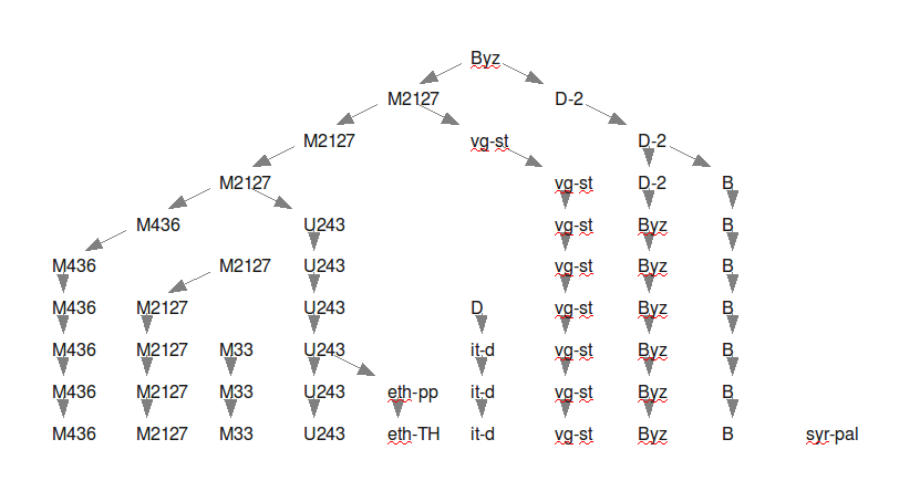
This series of partitions has some remarkable features. The first level, containing all of the witnesses, is a reminder of the unity of the text. The second level is surprising because it groups “Byzantine” (e.g. K, L) and “proto-Alexandrian” (e.g. P46, B) witnesses in the “Byz/D-2” cluster, while placing “secondary Alexandrian” (e.g. A, C) and “Western” (e.g. Old Latin) witnesses in the “Byz/M2127” cluster. The “Byz/D-2/B” and “Byz/D-2” clusters do not separate until the fourth partition, after the “Byz/M2127” and “Byz/M2127/vg-st” clusters split at the third partition. That is, the “Byz/D-2/B” (“proto-Alexandrian”) and “Byz/D-2” (“Byzantine”) clusters have more in common with each other than they do with either the “Byz/M2127/vg-st” (“Western”) or “Byz/M2127” (“secondary Alexandrian”) clusters!
At the fifth partition, the “Byz/M2127/U243” cluster forms and what remains of its parent cluster adopts a new medoid to become the “Byz/M2127/M436” cluster. At the sixth partition, a new cluster forms with M2127 as its medoid, drawing members from all but one of the clusters found in the preceding level. Nevertheless, it has much in common with the “Byz/M2127” cluster which split at the fifth level of partitioning so its top-most node has been placed directly beneath this ancestral cluster. The “D/it-d” and “M33” clusters are other orphans with a measure of connection with the ancestral clusters located directly above them. As the four members of the “syr-pal” cluster come from as many different ancestral clusters, this cluster is not placed beneath any others.
The process of subdivision is quite enlightening as it shows where various classes of witnesses fit into the overall scheme of things. To illustrate, the Ethiopic version turns out to be a distinct entity which separates at the ninth level. Prior to that, it resides in the “Byz/M2127/U243” cluster which includes U243, M365, M1739, and M1881. The supposed Syriac influence may therefore be illusory, the Ethiopic instead being founded on Greek texts which have numerous points of contact with the Peshitta.
Some clusters do not emerge until late in the process, but when they do they are intriguing. Previously unsuspected associations appear, such as the “syr-pal” cluster, including U44, U150, and syr-p. Could this represent a Syro-Palestinian text? The “M33” cluster is another interesting one, including Alexandrinus and Sinaiticus but nothing else apart from the modern construct which is the UBS text. Finally, the “M2127” cluster deserves a mention. Along with M6, M256, M263, and M1573, it includes the Coptic and Harclean Syriac. This could be an Egyptian constellation, but distinct from other clusters with a possible Egyptian provenance such as “M33”, “Byz/D-2/B”, and “Byz/M2127/M436”.
It is important to ask whether the clusters revealed by the foregoing analysis are real or whether they might instead be random fluctuations in the density of witnesses in textual space. This question can be explored by generating random data, subjecting it to the same analysis, then considering whether the two sets of results are inherently different.
To generate random data, a number of “pseudo-witnesses” can be manufactured using probabilities obtained from the data matrix of actual witnesses. If the variation units are independent of one another then the probability of a particular reading of a particular variation unit is best estimated by that reading's relative frequency within the variation unit. If they are not independent then it is necessary to consider other variation units and their readings when calculating a probability. It seems reasonable to assume that the variation units given in the UBS apparatus are independent with respect to internal considerations such as grammar or theology. That is, one does not expect the reading in one variation unit to play a determining role in the reading of another. It may be that there is a characteristic set of readings for a witness of a particular type which can be attributed to common ancestry. However, this is an external factor that is not based on any inherent property of the variation units. By contrast, it is not safe to assume independence of binary variation units extracted from multistate ones. Instead, internal correlations between the readings in such a binary set should be expected. Consequently, only the multistate data matrix will be used to obtain probabilities for this investigation, and only multistate pseudo-witnesses will be generated.
The script named
random.r
generates a specified number of pseudo-witnesses using relative
frequencies of readings extracted from an input data matrix of actual
witnesses. Below is a data matrix of pseudo-witnesses generated with this
script using the multistate UBS Hebrews data matrix as input. This data
matrix comprises sixty pseudo-witnesses, which is the approximate number
of witnesses included in the principal MDS maps obtained directly from the
actual multistate data matrix.
| Data set | Multistate |
|---|---|
| Random | → |
The following table provides three-dimensional MDS maps respectively produced from actual data and this randomly generated data. Maps in the first row are plain point clouds while those in the second include confidence regions.
| Type | Actual | Prop. of var. | Random | Prop. of var. |
|---|---|---|---|---|
| Plain | → | 0.417 | → | 0.210 |
| Confidence regions | → | 0.417 | → | 0.210 |
At first sight, there does not seem to be much difference between the two classes of maps. The randomly generated witnesses do seem to be more uniformly distributed. However, the difference is not so compelling as to dispel suspicion that the actual witnesses are distributed in the same way as their randomly generated counterparts. This is reminiscent of the similarity of the distribution of numbers of agreements for actual and randomly generated witnesses noted at the end of chapter three.
One clear difference is in the proportion of variance figure for the two classes. Three dimensions account for only 21 percent of the total variance among the random witnesses. By contrast, the figure for actual witnesses is almost twice as much, at just less than 42 percent. That is, the actual data has a lower dimensionality than the randomly generated data, making it easier to squeeze into only three dimensions.
Clustering of the two classes of witnesses can be compared in a similar way. The following table shows results obtained when the randomly generated witnesses are divided into one to ten clusters:
| Level | Clusters | ||||||||||
|---|---|---|---|---|---|---|---|---|---|---|---|
| 1 |
|
||||||||||
| 2 |
|
||||||||||
| 3 |
|
||||||||||
| 4 |
|
||||||||||
| 5 |
|
||||||||||
| 6 |
|
||||||||||
| 7 |
|
||||||||||
| 8 |
|
||||||||||
| 9 |
|
||||||||||
| 10 |
|
The figure below represents these partitions with the same kind of directed graph as used above for the actual data:
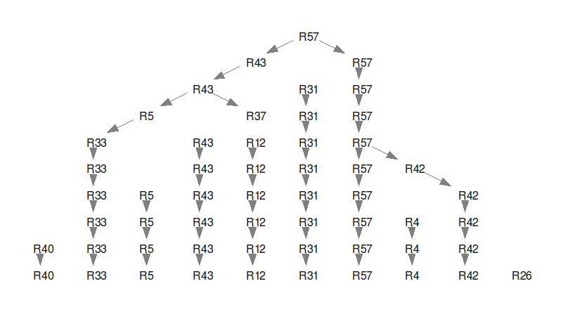
There does not seem to be much difference between the partitioning observed in actual data and that seen when random data is subjected to the same process. There are more orphan clusters, although several trials of this kind would be needed to decide whether this is just a quirk of the trial performed here. A clear distinction is that the number of members per cluster at a given level of partitioning is more uniform for random than for actual data. For example, the numbers at the tenth level of partitioning range from two to sixteen for the actual data but three to nine for the random data.
A statistical test would need to be performed in order to confirm that there is a substantive difference between results obtained when subjecting actual data on one hand and randomly generated data on the other to this kind of partitioning exercise. I do not know how to do such a test but suspect that if one were done a real difference would be found. Nevertheless, as with the distributions of numbers of agreements presented at the end of chapter three, the actual data seems to share at least some of the characteristics of randomly generated data. The sample used in this study is small and upon analysis produces correspondingly ambiguous results. It may be that analysis of a larger sample would reveal more pronounced differences between actual and randomly generated data.
| Note |
|---|---|
The similarity of results obtained with actual witnesses and randomly generated ones should not be taken to mean that the actual witnesses contain a random text. Instead, it means that the sample examined here is not unlike one that would result if the reading of each witness at each variation unit were chosen at random from the readings that exist at those places, as might be expected to happen if the number of witnesses is small compared with the original population. |
Another reason for doubting the authenticity of observed clusters is that choosing a different clustering technique can produce different results. Whereas the “optimal partitioning” method has been used in this chapter, any of the others described in chapter four could have been used. (The name of the “optimal partitioning” method should not be taken to mean that it is better than the others. Each has its own strengths and weaknesses.) As noted in chapter four, there are similarities between the groupings obtained when different clustering techniques are applied to this data, but no consensus. In order to be sure that observed clusters were real, they would have to persist when other partitioning techniques were employed.
Finally, including a tight cluster of witnesses can cause an islanding effect in MDS maps which isolates the cluster and distorts the entire point cloud relative to the configuration it would have if only one member of the cluster were included. To illustrate, the data matrix presented here is a copy of the random data matrix with three copies of pseudo-witness R7. The first, R7a, is an exact copy of R7 while the other two, R7b and R7c, have been changed to have a different reading to the original in the first variation unit alone. A three-dimensional MDS map based on this data matrix is shown here. Comparing it with the corresponding map derived from the original random data matrix shows the islanding effect. The introduced pseudo-witnesses R7a, R7b, and R7c form a tight cluster while R7b and R7c displace the rest of the witnesses from the locations they would have had if these two had not been included. (Being an exact copy of R7, R7a does not displace the others.) This islanding effect acts to exaggerate the appearance of clustering if a few very similar witnesses are present. Clusters in the MDS maps produced from the UBS data are affected by the islanding effect. To give a particular example, the “Western” cluster containing Old Latin and Vulgate witnesses would not be as distinct from the “secondary Alexandrian” cluster containing witnesses such as C, M81, and M2464 if the former did not contain as many very similar witnesses.
What forces gave rise to the observed clusters, if in fact they are real? Were they temporal, geographical, recensional, political, theological, or merely random? Probably, they were all of these, and more besides. Whatever their nature, they acted through individuals to produce the copies which survive today. The actions of copyists eventually resulted in the formation of texts that served as exemplars for various copying locations at different times in history.
Typically, one exemplar was used when making a copy. More than one exemplar could have been used, but this would not have been the normal mode of operation. As the scribe copied, errors would have been made. (Anyone who doubts this need only ask a room full of people to copy a text by hand.) A scribe may also have substituted readings from sources besides the exemplar, which sources may have been another exemplar or the scribe's mind. Errors are unintended; substitutions may be intentional or not. (An example of an unintentional substitution would be unconscious replacement of a less familiar phrase with a more familiar parallel when the text is in the scribe's mind between being read and written down.) The changes that make texts diverge can thus be divided into two classes: intentional and unintentional.
Unintended changes are random in nature, having no particular direction in textual space. Nevertheless, randomness does not imply zero net change. To illustrate, a one-dimensional “random walk” experiment involves discovering the net displacement after a number of steps where each step has an equal probability of being to the left or right. If, say, five steps were allowed, the final position could be anywhere between five steps to the left or five to the right of the start. Typically, the position would be somewhere closer to the start, but is more likely than not to be somewhere besides the start. In the same way, unintentional errors cause net movement away from the exemplar. As the errors of a number of generations of copies accumulate, the movement becomes more pronounced. The direction of drift through textual space caused by unintentional change is hard to predict, being towards regions that correspond to the kinds of unintentional change produced by scribal nature.
Intentional changes have the same effect of causing a net displacement between exemplar and copy. In contrast to unintentional changes, the direction of movement in textual space caused by intentional changes is easier to predict. If a scribe is aiming to correct a first text so that it conforms to a second one then the result will be somewhere between the former and latter; how thoroughly the corrector works determines where the result lies along the line between the first and second texts. If the changes are recensional, so that the scribe has become an author, then the result will be a new text that is displaced from its model in a direction through textual space that corresponds to the author's intent. Typically, the drift away from an ancestral text is gradual, moving in small steps from one generation to the next. Sometimes, however, a great leap can occur, as when an editor sets out to create a recension or when one text is corrected against a very different one.
The three-dimensional principal MDS map for binary data displays a number of these kinds of textual development. The second corrector of Codex Claromontanus (D-2) did a thorough job of conforming the text to a Byzantine model. However, the result seems to have overshot the mark. Possibly, the model used by the corrector was in the vicinity of the result, although the difference may also be due to sampling error. Another example is the Armenian version, which through editorial action moved from its presumed place of origin near the first Georgian (geo-1) to the “Byz/M2127/M436” cluster.
Besides migrations that shift a text from one cluster to another, there are those that end in a location between two or more clusters. To give a few examples, M1739, syr-pal, and geo-1 all lie between the “Byz/D-2/B” cluster on one hand, and “Byz/M2127/vg-st” cluster on the other, but are also pulled towards other regions of higher density. These may represent transitional forms: mixtures of readings selected from two or more families of texts known in the physical locations where they were produced. If M1739 is similar to Origen's text then its textual location indicates that Origen used a text which reflected aspects of a number of the textual families current in his time.
Finally, there is the phenomenon of textual divergence. Each of the clusters identified above has a notional centre, and the locations of these centres differ. Thus, for example, the “Byz/M2127/vg-st” cluster, whose origin presumably goes back to the first Latin translation, lies in a different part of textual space to the “Byz/D-2/B” cluster, whose origin may go back to a European or Egyptian production of the Greek text. Divergence, which is movement of one textual centre away from one or more others, is caused by a set of witnesses developing a distinct set of readings. Instead of favouring readings that another cluster already possesses, and thereby moving towards it, a divergent cluster prefers a combination of readings not held by other clusters, thus moving away from them all.
The maps show a number of regions of higher density. These might point to a corresponding set of popular archetypal texts that copyists sought as exemplars. How these archetypal species arose is not known. It may be that in the earliest phase of textual propagation each Christian population centre had its own species of text, one that differed significantly from others because the very first generation of copies was sent to isolated centres that did not compare their texts until a number of generations of copies had been made. Another possible cause of archetypal divergence is translation, as with the Old Latin and Syriac. Yet another is accretion of “improvements” that sought to smooth roughness, ease difficulty, conflate diversity, and make sense of primitive corruption. If the various centres copied their texts predominantly from local exemplars then each centre would tend to develop its own distinctive text. Once established, only major events such as widespread textual destruction or adoption of an authoritative standard would be able to displace these regional texts. Even if the regional texts were displaced, we might expect some of their descendants to have survived. The areas of higher density evident in the textual maps may well be the remnants of such archetypal texts.
Darwin's theory has an application here, although whether it is practically useful remains to be seen. “Natural selection” would tend to favour those readings best adapted to the then current scribal climate. The reading which is by nature best adapted to survive the scribal “read, remember, (think), write” loop is more likely to propagate. (The “think” part would apply if the scribe were thinking critically about which reading to select, as occasionally happened.) Thus, part of the textual researcher's task is to go against the flow of this selection process to identify primitive readings which have been dethroned by scribal nature.
Having seen the distribution of surviving witnesses through textual space, one is curious to know where the original text would have been located. As discussed by Epp, one needs to be careful when using the word “original” to describe the earliest form of a New Testament writing ([Epp 1999]). Some writings (e.g. Mark and Romans) bear the marks of early editors while others (e.g. Ephesians) may have begun as “circular” letters, having been distributed to a number of places simultaneously. The Epistle to the Hebrews, however, does not have any of the additions, deletions, substitutions, dislocations, or transpositions of large sections of text that would make it difficult to talk about an original text. Neither is there reason to believe that Hebrews was originally sent to anyone besides the group for whom it was written, with personal notes attached. In the absence of evidence to the contrary, the idea of a single “original” text for Hebrews remains the simplest and, therefore, best hypothesis.
Given that there was a single original of Hebrews from which all our copies are descended, where should it be located? If the UBS editors have managed to reconstruct the original text of Hebrews then it would be located where the UBS text lies. The partitioning exercise indicates that this is in the “M33” cluster, along with surviving witnesses M33, Sinaiticus, and Alexandrinus. However, it is fair to say that few contemporary students of the text would place the original here. Many would instead be inclined to locate it in the “Byz/D-2/B” cluster comprised of P13, P46, and B. These are, after all, our oldest and, perhaps, best surviving witnesses. Another possibility would be to locate the original near the centre of mass of the surviving point cloud, somewhere near U150. Yet another possibility would be to locate the text at the centre of the Byzantine cloud, or at the centre of another one of the clusters which emerge from the partitioning exercise.
Actually, the kinds of analysis conducted so far in this study do not shed any light on where the original might be located. Being exploratory in nature, they serve only to reveal the distribution of surviving witnesses, not what caused the distribution to take this form. A genetic analysis is required to map the descent of texts, working backwards from surviving witnesses to intermediate forms and finally to the original. Whether or not such an effort can succeed depends on factors such as how representative the survivors are of the entire tradition, the proportion of survivors relative to the total number that ever existed, and the reliability of the scribal transmission system. Topics such as these will form the content of the chapters to follow.
At this point I would like to sketch one scenario by which a text such as the Epistle to the Hebrews might have been transmitted to us. We begin with the original text as written down by whoever we have to thank for it. It may have been corrected by the author, immediately introducing fodder for textual variation. Next, it was carried to the recipients who, in the case of Hebrews, seem to have been a single group, possibly in Rome. (Another writing such as Ephesians might have been initially copied for a number of Christian communities.) Once received, Hebrews was kept and copied for the edification of others. At some point it was incorporated into a collection of Paul's letters, possibly by the end of the first century ([Zuntz], 13). Whether as a single letter or in a collection, Hebrews was transmitted from its original destination to various communities around the Mediterranean rim. Every copying event in this and subsequent steps had the potential to introduce changes.
In the first generations of copies, Christian communities were relatively isolated. While it was not difficult to carry a letter from one side of the Empire to another, if a Christian community needed a copy then it would be easier to obtain an exemplar from nearby than far away. Thus, the principle of least effort would tend to favour selection of a local exemplar from which to make a copy. The relative isolation of the far-flung Christian communities would tend to favour development of a local species of the text in each geographical centre. Textual variations peculiar to each centre would remain there due to the tendency to use local exemplars. Each centre would thus develop its own population of variation units and readings. Astute readers would compare manuscripts and note differences, correcting the manuscripts here and there. However, as long as they were comparing local manuscripts, the local population of readings would retain a distinctive character. Readings could have been transmitted from one centre of copying activity to another at any stage of the process. However, the frequency of transmission of these “viral” readings would be relatively low while the centres remained isolated. As communication increased, so did the flow of readings.
At some point it became apparent to Church authorities that there was significant variation in the New Testament writings, and efforts towards standardization began. It may be that the process which eventually produced the Byzantine standard text began in this way. This text may be a recension drawn from a number of diverse texts known to whoever produced its first examples. Alternatively, it may be descended from a single textual cluster. If so, and if the apparent geographical associations noted above are real, then the Byzantine standard text seems to be based on an ancient text associated with Antioch and Syria. If, on the other hand, the Byzantine standard were extracted from a number of diverse archetypes then its location in textual space should lie between more primitive textual clusters. However, the maps produced here show that the Byzantine textual cloud is centred away from the centre of mass of the point cloud formed by all surviving witnesses, indicating that it is not based on a recension of diverse texts.
The high level and large scale efforts required to produce the fifty Bibles commissioned by Constantine for his new capital may have been what made Church authorities aware of the existing diversity of texts among its various geographical centres and prompted them to strive for a standard text. (The circumstances surrounding Jerome's recension of Old Latin manuscripts to produce the Vulgate tell us that this kind of thinking was current in the fourth century.) This is not to say that the fifty were the first examples of the Byzantine standard text. Instead, they probably would have been copied from exemplars available in or near Caesarea. One might expect these fifty to have left their mark on surviving evidence. While only a very tenuous indication, the presence of the Armenian version points to the “Byz/M2127/M436” cluster being their descendants.
Returning to the question of where the original should be located in textual space, a likely contender is the place associated with the initial point of dissemination, possibly Rome. If one of the apparent clusters seen in the MDS maps can be identified with Rome then this would be a suitable place to locate the original text. The age of P46, its placement of the Epistle to the Hebrews second only to the Epistle to the Romans, and the apparent proximity of the text of P46 to that used by Ambrose of Milan hint that P46 preserves an early Roman text. If so then the kind of text found in witnesses belonging to the “Byz/D-2/P46” cluster has a claim to being our closest approximation to the original. Then again, the location from which the earliest generation of copies disseminated could have been any other centre. Just as no one is quite sure where Hebrews was originally sent, so the earliest centre of its dissemination is unknown. Only God knows who wrote Hebrews and from where it was first broadcast.
Analysis of variant textual data presented in the UBS apparatus of the Epistle to the Hebrews reveals what appear to be concentrations of witnesses in the “textual space” they occupy. While the MDS maps and partitions derived from the apparatus data show what seem to be real differences from randomly generated analogues of actual witnesses, it would take a statistical test to conclusively demonstrate that these concentrations are more than random fluctuations.
If the sample of variation units and witnesses contained in the UBS apparatus are representative of the entire tradition then the distribution of witnesses seen in the MDS maps produced in this chapter reveals the actual shape of the great cloud of witnesses that once existed. Potential causes for the cloud having the shape it does are manifold. The distribution of witnesses has been affected by many factors and events including time, geography, translation, large scale copying efforts, standardization, and, not least, scribal nature.
The mapping and partitioning techniques employed so far provide insights into the relationships and distribution of surviving witnesses. Analysis of a larger sample would produce more accurate results. However, none of these techniques is much help when it comes to identifying the most primitive text. Some circumstantial evidence suggests that the original was a text of the kind preserved in the “Byz/D-2/B” cluster.
[UBS] Aland, Barbara, Kurt Aland, Johannes Karavidopoulos, Carlo M. Martini, and Bruce M. Metzger, eds. 1993. The Greek New Testament. United Bible Societies, 4th rev. ed. Stuttgart: Deutsche Bibelgesellschaft.
[ECM] Aland, Barbara, Kurt Aland†, Gerd Mink, Holger Strutwolf, and Klaus Wachtel, eds. 1997-. Novum Testamentum Graecum: Editio Critica Maior. Stuttgart: Deutsche Bibelgesellschaft.
[Aland and Aland] Aland, Kurt and Barbara. 1989. The Text of the New Testament: An Introduction to the Critical Editions and to the Theory and Practice of Modern Textual Criticism. 2d rev. ed. Trans. Erroll F. Rhodes. Grand Rapids: Eerdmans.
[Alexanian] Alexanian, Joseph M. 1995. “The Armenian Version of the New Testament.” In The Text of the New Testament in Contemporary Research: Essays on the Status Quaestionis. Ed. Bart D. Ehrman and Michael W. Holmes. Studies and Documents 46. Grand Rapids: Eerdmans, 157-72.
[Chatfield and Collins] Chatfield, Christopher and Alexander J. Collins. 1980. Introduction to Multivariate Analysis. London: Chapman and Hall.
[Cox and Cox] Cox, Trevor F. and Michael A. A. 2001. Multidimensional Scaling. 2d ed. Florida: Chapman and Hall.
[Everitt] Everitt, Brian S. 2005. An R and S-PLUS Companion to Multivariate Analysis. London: Springer.
[Epp 1991] Epp, Eldon J. 1991. “New Testament Papyrus Manuscripts and Letter Carrying in Greco-Roman Times.” In The Future of Early Christianity. Ed. B. A. Pearson. Minneapolis: Fortress Press, 35-56.
[Epp 1999] ———. 1999. “The Multivalence of the Term 'Original Text' in New Testament Textual Criticism.” Harvard Theological Review 92, 245-281.
[Finney 1999] Finney, Timothy J. 1999. “ The Ancient Witnesses of the Epistle to the Hebrews: A Computer-Assisted Analysis of the Papyrus and Uncial Manuscripts of ΠΡΟΣ ΕΒΡΑΙΟΥΣ. ” PhD dissertation, Murdoch University. http://purl.org/tfinney/PhD/.
[Finney 2002] ———. 2002. “ What Agreement Is Not. ” In “What Does the Text Actually Say?” A Festschrift in Honour of Dr Richard K. Moore. http://www.halotype.com/RKM/.
[Finney 2003] ———. 2003. Manuscript Copying Simulation. Online resource. http://rosetta.reltech.org/TC/downloads/simulation/.
[Friberg and Friberg] Friberg, Barbara and Timothy (eds). 1981. Analytical Greek New Testament. Grand Rapids: Baker Book House.
[Lake] Lake, Helen and Kirsopp. 1911. Codex Sinaiticvs Petropolitanvs: The New Testament: The Epistle of Barnabas and the Shepherd of Hermas. Photographic facsimile with an introduction by Kirsopp Lake. Oxford: Clarendon Press.
[Lyon] Lyon, Robert W. 1958. “A Re-examination of Codex Ephraemi Rescriptus.” Ph.D. dissertation. University of St Andrews.
[Metzger 1977] Metzger, Bruce M. 1977. The Early Versions of the New Testament: Their Origin, Transmission, and Limitations. Oxford: Clarendon Press.
[Metzger 1992] ———. 1992. The Text of the New Testament: Its Transmission, Corruption, and Restoration. 3d enlarged ed. New York: Oxford University Press.
[Milne and Skeat] Milne, H. J. M. and T. C. Skeat. 1938. Scribes and Correctors of the Codex Sinaiticus. Oxford: Oxford University Press.
[Moore and McCabe] Moore, David S. and George P. McCabe. 1993. Introduction to the Practice of Statistics. 2d ed. New York: W. H. Freeman.
[Petzer] Petzer, Jacobus H. 1995. “The Latin Version of the New Testament.” In The Text of the New Testament in Contemporary Research: Essays on the Status Quaestionis. Ed. Bart D. Ehrman and Michael W. Holmes. Studies and Documents 46. Grand Rapids: Eerdmans, 113-30.
[Pierce] Pierce, John R. 1980. An Introduction to Information Theory: Symbols, Signals, and Noise. 2d rev. ed. New York: Dover Publications.
[R Project] R Development Core Team. 2005. R: A Language and Environment for Statistical Computing. Vienna: R Foundation for Statistical Computing. http://www.R-project.org/.
[Souter] Souter, Alexander. 1954. The Text and Canon of the New Testament. 2d ed. revised by C. S. C. Williams. London: Gerald Duckworth.
[Streeter] Streeter, Burnett Hillman. 1930. The Four Gospels: A Study of Origins Treating of the Manuscript Tradition, Sources, Authorship, and Dates. Rev. ed. (8th impression, 1953). London: Macmillan.
[Thorpe] Thorpe, J. C. 2002. “ Multivariate Statistical Analysis for Manuscript Classification. ” TC: A Journal of Biblical Textual Criticism 7. http://rosetta.reltech.org/TC/vol07/Thorpe2002.html.
[Ubuntu] Ubuntu Linux. Operating system. http://www.ubuntu.com/.
[Venables and Ripley] Venables, William N., and Brian D. Ripley. 2002. Modern Applied Statistics with S. 4th ed. New York: Springer.